
Reproducing the goal: The Calibration Set is more beautiful, can it be brought to the next set of samples?
The previous experiment shows that dozens of samples may push the temperature to the search boundary. This article adds another controlled question: if the calibration function is allowed to bend and form a platform, is it more reliable than the temperature scaling with only one parameter? We fixed the model, original prediction, calibrated identity and audit identity, and only replaced the post-processing method, while retaining a small pre-registered small sample condition.
The answer given in this actual verification is no, but the scope is limited: when using the complete 256 calibration samples, the loss of order-guaranteed regression is lower in the fit data, and the 360 audit samples do not exceed temperature scaling ; it also assigns a deterministic error probability to seven wrong answers. This is a recalculation method experiment, not the method ranking on all datasets, nor is it open to generate reliability.
Core idea: a knob with a curved curve
temperature scaling only changes the distance between the scores of the two categories. The positive temperature does not flip the size relationship, so the category prediction remains the same. Sequence-preserving regression looks for a non-decreasing map: a sample with a greater probability of the original class, and the probability of the positive class after calibration cannot be smaller; but the adjacent sample can fall on the same platform. The "order-preserving order" here allows parallelism, which does not mean that all sorting is strictly preserved, and it does not guarantee that the original classification threshold will remain valid.
In the paper report, Guo, Pleiss, Sun and Weinberger found in a 2017 study that the single parameter temperature scaling is effective in its many experiments. This is the reason for choosing a simple control, not an alternative evidence for the results of this experiment. Papers and Meeting Minutes
The official document defines the order-preserving regression as the least square problem with a monotonous constraint, and reminds that the calibration sample should be paid attention to overfitting. Here we call the official implementation of the fixed version directly, instead of approximating the teaching as the library. Sequence regression document、Probability Calibration Document
Formulas and Evaluation Objects
For each input, the model produces two original fractions, that is, logits. remember them as , the main class is labeled as , the score difference is . The temperature is converted to:
here is the probability of a positive emotional category, is a scalar fitted on the calibration subset; the model batch output shape is , the post-processing probability vector shape is . We inherit the bounding inverse temperature solver and use the Calibration Set Negative Log-likelihood to determine the parameters, and the boundary and iterative rules are not dependent on the audit results.
Order-guaranteed regression uses the original normal class probability As the absciss, look for the map :
is the number of samples of this fit, is the calibration probability of the sample. The function constraint direction is explicitly set to increment, and the program is not automatically selected according to the relevance. The two methods have different optimization goals, so this is the overall comparison of commonly used methods, and cannot be interpreted as pure causal experiments that only increase the number of parameters.
The main indicators are the double-category sum Brier score, that is, the square distance between the probability and the label:
is the number of evaluation samples, It is the positive-class probability of a method output; the error of factor 2 from the two categories is added. The auxiliary indicator is Negative Log-Likelihood, that is, NLL. For the true zero-true class probability, the loss in mathematics is infinity. In order to still be able to compare limited tables, the protocol is additionally preset , only limit the true class probability to . Fit, Brier, classification and boundary counting always use untruncated probability.
A guide to the official implementation
Read the pinned commit first IsotonicRegression._build_y: it sorts the inputs, merges duplicate x-values, performs a weighted isotonic fit, and removes redundant points on plateaus that do not affect predictions. Then read _build_f and _transform: the official implementation predicts by interpolating linearly between retained knots. For inputs outside the calibration range, this experiment explicitly chooses to clip to the endpoint values. A staircase is a useful mental picture of an isotonic fit, but making the prediction constant on every interval would implement a different rule. Fixed source code
This time, the real submission corresponding to the corresponding version 1, 6.1 is verified, and the module is confirmed to be installed by byte by byte, which is consistent with the official file. The tag object is different from the commit object. The first time it is directly used to read the file with annotated tag and returns does not exist, and the actual submission is successfully resolved; the failure is kept in the verification record. The source map distinguishes the official library call and inherited self-written temperature solver and independent recalculation script. The license is the official BSD three clauses and the license recorded by each inheritance module.
Minimum experiment: same data, same model, different mapping
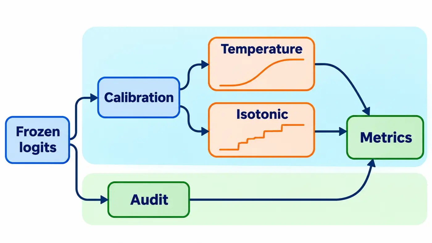
The model continues to use the fixed DistilBERT SST-2 checkpoint; the data continues to use the official Validation identity list. The original division is fixed according to the identity hashing, the exploration pool 256 articles, the calibration pool 256 articles, and the agreement audit pool 360 articles do not intersect with each other. This article only reuses the real logits saved in the previous two pools, and does not re-screen the sentences, and does not add semantic annotations.
SST-2 has been used in historical experiments, and the audit results are also observed in the first two articles. Therefore, the "independent" here only means that the current calibration fit is not entered and cannot be written as a test set that has never been seen before. IMDb Sanchi did not reason this time, and finally confirmed that the pool remained unused.
In this article, the identity sorting rules are pre-frozen, and the first thirty-two and complete articles of the hash are formed to form nested conditions. The temperature and sequence regression are fitted at the same time for each condition, and the original probability of the original probability control is completely output. See more typical cases without changing the seeds, and do not select the sample size, mapping or truncation parameters according to the audit. The thirty-two articles are exactly predicted to be correct.
Run the existing fixed model cache, verify the file hash first, then execute eight real CPU test runs, and re-acquire the output in the shape of eight rows and two columns. The formal method compares and reuses the prediction of the 616-point historical model; it cannot be called the re-complete 616 model forwards today. This new analysis and actual measurement is about 0.025 seconds, and the peak memory of the process is about 96 MiB; eight test runs forward about 0.075 seconds, and the imported process is about 0.548 seconds. The complete environment and memory records are saved with the source code. The download and use the caching cache, this time does not report the new download time-consuming. The newly added are four fits, twelve sets of evaluations and independent arithmetic verification, no model training or paid calculations.
Results: Lower fitting errors did not translate into better audit performance
The following tables are the actual results of 360 audit samples. NLL columns use preset truncation rules, and all methods share the same denominator; untruncated sequence-preserving NLL is infinite at both sample sizes.
| calibration amount | Method | Brier | truncated NLL | Number correct |
|---|---|---|---|---|
| Don't fit | raw probability | 0.154001 | 0.384113 | 330 |
| 32 | temperature scaling | 0.166945 | 1.145233 | 330 |
| 32 | Guaranteed regression | 0.154905 | 0.614199 | 330 |
| 256 | temperature scaling | 0.135151 | 0.237136 | 330 |
| 256 | Guaranteed regression | 0.137395 | 0.420606 | 329 |
On the complete calibration pool, the preservation regression fits the Brier of 0.115867, which is lower than the temperature scaling 0.147385; the order of the audit set is reversed. Its audit output is 249 at zero or one, and seven of them have zeroed the probability of the real category. When the temperature is about 2.4819, the output has no boundary probability. This means that you can't just look at whether the Calibration Set curve fits the label, and you can't just report the limited NLL after the truncated.
Small sample conditions are more worthy of preservation. All thirty-two articles are all correct, and the temperature is pushed to the lower bound of 0.05; Both of the audit sets are inferior to the original probability. There are eleven true classes with zero probability, but Brier only slightly deteriorates: square losses are bounded, and the logarithmic loss is extremely sensitive to absolute errors. The two answer different questions.
The small sample results of temperature also expose the numerical trap. Limited logits and positive temperatures do not generate precise zero probability mathematically, but floating-point sigmoid can be rounded to one, and then subtracting it will get zero. Therefore, a clearly marked post-mortem numerical diagnosis is added: use stable softplus to directly calculate the NLL from logits. This condition is stable and untruncated NLL is 7.271314, which is still poor but limited. It does not change the main indicator of the pre-registration, does not re-select the temperature, and does not falsely report the rounding event into an infinite mathematical loss.
Failure investigation and independent recalculation
Start by checking sample identities. Both methods should use exactly the same calibration IDs, with no overlap between calibration and audit, and the input hashes should match the protocol. Next check which probability is being calibrated. Here it is the probability of the positive class. Substituting the maximum class confidence changes what the label means. Finally, inspect interpolation and extrapolation, especially the handling of repeated x-values and predictions outside the calibration range.
The independent audit does not call the official fitter again, but uses the interval average, minimum and maximum expression of the minimum squares of the sequence protection sequence to reconstruct the fit value, and then interpolates independently, and checks all outputs and indicators item by item. The maximum probability difference is about one multiplied to the negative sixteenth power. The model test run is also compared with the historical eight outputs by identity, and the floating-point errors with records are allowed, but the categories are required to be consistent. Arithmetic auditing is not a manual label review; this article does not produce new semantic labels that require real person judgment.
Code and instructions for reproducing the results
The public fixed version has been verified: Source directory、README、SOURCE_MAP. The package includes a unified entry, official model download and test scripts, fixed dependencies, configuration, protocol, source map, sample-by-sample derivative results and audit scripts. The minimum running command is:
python -m pip install -r requirements.txt
python run.py
python audit.py
Expected to generate results.json、analysis_environment.json and audit_result.json. Executes separately when the model cache is available python model_run.py smoke --cache .cache; the first use of the corresponding run prepare command. The download requires about 270 megabytes of model resources, the default CPU is four threads, and the budget is 30 minutes and six GiB memory. The original sentence is not distributed with the package due to the unclear license of the data card. Download the script to fix the official revision, and the existing cache must pass the hash check.
Another place that is easily confused is the tag threshold. temperature scaling is still classified by the positive and negative of the original score difference, but the order-guaranteed regression may move the probability that the probability exceeds one-half, and the platform will also be manufactured. The unified agreement in this article is strictly greater than one-half to predict the positive class, and the negative class is predicted when it is equal. Therefore, the correct number of correct numbers has dropped from 330 to 329 under the condition of the complete pool, which is the result of the actual mapping and threshold values.
Similarly, large audit sample size does not automatically mean more reliable. The two methods share the audit sample, and the loss difference is a paired observation; this article does not construct the interval for the difference value, and does not make a significant test of multiple groups of candidates. The Brier difference of around 0.002 can only be used as a description of this fixed sample. Boundary errors are more suitable to help put forward the next hypothesis, and cannot replace the verification of cross-divided and cross-data domains.
Checkable follow-up questions and summary
My interpretation is that, in sparsely populated score ranges with no observed errors, a flexible mapping can mistake a locally pure sample for certainty. One fixed small subset and one full pool cannot tell us how often that happens or establish a general winner. A follow-up comparing smoothed isotonic regression, probability clipping, or larger calibration sets would need its own prespecified candidates and selection rule. Repeatedly using this audit to pick the best combination would forfeit its status as an independent evaluation.
The next article changes the class proportions in the calibration set to see how well one global temperature serves both classes. The conclusion we can check here is narrower. On the same data, reducing fitting error does not guarantee better probability estimates on the audit set. A probability at the boundary must be distinguished from a value rounded to it. The number of correct classifications, squared loss, and log loss each measure something different. These failures belong in the record for the next study.
References
Search and source code verification date: 2026-11-04.
- Guo, C., Pleiss, G., Sun, Y., Weinberger, K. Q. 2017. On Calibration of Modern Neural Networks,ICML / PMLR 70.
- scikit-learn official: Isotonic regression and Probability calibration. Dynamic documents are only used as conceptual sources, and the actual execution version is fixed to 1.6.1.
- scikit-learn 1.6.1: Pinned commit source code.
- DistilBERT fixed model card.
- SST-2 fixed data version.
Apps by the author
The following is the author's own product promotion. In addition to the research blog, I also independently develop daily gadgets: Daily Expense Journal Used to record revenue and expenditure, budget and savings objectives; One Small Action Help choose small actions according to time and energy, and record the feelings after completion. Welcome to your own needs, you can also go to Personal website Read more articles and work introductions. These products are not endorsed with this paper, experimental results and research institutions.