Reproducing the target: a parameter will also be biased by the small sample
In the previous article, on a fixed two-classification model, 256 calibration samples were used to fit the temperature of about 2.48, and the Negative Log-likelihood of the audit set decreased. It is easy to generate an intuition according to this: since there is only one parameter, dozens of marks should be enough. Today, I only test this intuition, do not change the model, do not try new calibration methods, and do not pick out the best performing random seeds.
This actual verification found that among the fifty samples of the 16 samples, there are ten calibration subsets that happen to have no model errors. These ten fitting temperatures have all reached the preset lower bound, and after being applied to the same audit pool, the probability loss is significantly deteriorated. The question is not a sudden change in the classification answer, but the probability that the wrong answer is closer to one. This negative result shows that less parameters do not mean that the information provided by the data is sufficient.
The reviewable product of this article is 250 fitting records: each time contains sample identities, temperature, boundary marks, calibration errors, and audit losses. Conclusion is limited to fixed open models, fixed finite sample pools and current sampling protocols, and does not write a local experiment as a general sample size suggestion.
Core ideas: separate data fluctuations from optimization failures
temperature scaling is the logits of the classifier, that is, the category score before normalization, and then calculate the probability after uniformly divide it by a positive number. Guo et al. studied this post-processing method in a 2017 paper; the effectiveness of the paper report comes from its specific experiments and cannot replace the small-sample test of the current model.
Here the DistilBERT SST-2 checkpoint, tokenizer, tag mapping, truncation length and real prediction cache are frozen, and only the identities and amounts of the samples participating in the fit are changed. Repeat sampling of the same scale, you can observe how sensitive the estimator is to the composition of the sample. At the same time, use another numerical method to solve it independently to check whether the abnormal temperature is not converging, or whether the objective function does prefer the boundary.
The two interpretations are different in response. The algorithm error needs to be repaired and implemented; if there are not enough error samples in the data, the missing information cannot be filled several times. We do not adjust the temperature boundary after seeing the audit results, retain the original constraints, and facilitate the comparison with the previous article.
Formulas and Modules: Why Zero Errors Push Up Self-Confidence
antiward sample, set the two categories of scores as and , tags Take zero or one. Define score difference , inverse temperature , then the positive-class probability is
here is the temperature, is a positive scalar; the original output shape of each batch is , the probability still corresponds to two fixed emotional tags. It is not the correct probability of open text generation. Temperatures stay positive, so the size relationship of the two fractions will not be changed in theory.
The fitting goal is the average negative log-likelihood on the calibration subset, referred to as NLL:
is the number of samples used for this fitting. The implementation adopts a stable SoftPlus calculation to avoid large exponential overflow; the main solver uses the derivative dichotomy method, and the independent audit uses the golden segmented search, and does not import the main fit function.
The second formula shows that the target is convex to the inverse temperature. If all samples are strictly correctly categorized and each first derivative is negative, increasing the inverse temperature will continue to reduce the training target. Therefore, the best solution to the constrained temperature falls on the upper boundary of the inverse temperature, that is, the lower bound of the temperature. This is not evidence of "the model is really completely reliable", but rather the behavior of the objective function on the limited sample. If there are samples of equal or complete degradation, it needs to be discussed separately, and these situations will not be mixed into the explanation this time.
A minimal experiment and evaluation protocol
The 872 samples of the original validation have already been divided into fixed identity hashings: Exploration Pool 256 Articles, 256 Calibration Pools, and 360 Agreement Audit Pools. This article only reads the real logits of the previous calibration and audit. SST-2 has been used in historical projects, and the audit pool has also been observed in the previous article, so this is an exploratory method experiment, and it cannot be called a test set that has never been seen. The three pools of IMDb have not been visited this time.
Before calculating a new subset, we save the protocol with the input hash. Seeds are fixed at 11800 to 11849; each seed is sorted according to the SHA-256 number of the seed and sample number, and then the first 16, 32, 64, 128, 256 are taken. In this way, the small subsets in the same child are the prefix of the large subset, which is convenient for pairing and tracking. There is no layer by label or number of errors, and no subsets that are not ideal are deleted.
Fifty times each scale is fitted, and the inverse temperature range is used , two points and one hundred rounds; the temperature corresponds to the same value interval, but the upper and lower ends are interchanged. The main indicators are pre-determined as the standard deviation of temperature; at the same time, the median, range, boundary times, zero errors, and the NLL on the unified audit pool are reported at the same time. Audit results are not reflowed to the fitting step.
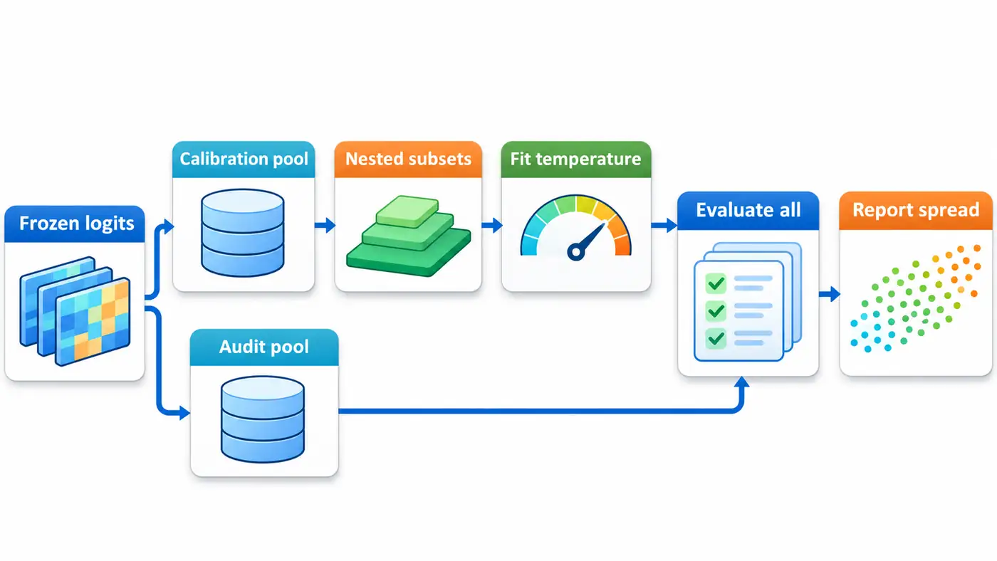
The figure is a schematic representation, and the terminal scattered point does not represent the measurement result. A total of 250 scalar fittings in the new experiment, without retraining the classifier. In addition, eight real CPU inferences are implemented, and the loading path of the cache and the current model is checked; all official statistics are still from the fixed 616 items that have been predicted, and the cache analysis cannot be recorded as a new model inference.
What we tested: the mean masks the boundary failure
| Calibration quantity | median of temperature | temperature standard deviation | temperature range | borders | Audit NLL median |
|---|---|---|---|---|---|
| 16 | 2.7254 | 1.4284 | 0.0500–5.3817 | 10/50 | 0.25797 |
| 32 | 2.6012 | 0.7061 | 0.0500–4.4586 | 1/50 | 0.24192 |
| 64 | 2.5430 | 0.3619 | 1.4686–3.3428 | 0/50 | 0.23881 |
| 128 | 2.5407 | 0.1994 | 2.1111–2.8738 | 0/50 | 0.23786 |
| 256 | 2.4819 | About zero | 2.4819–2.4819 | 0/50 | 0.23714 |
At the 16th rule, the temperature average is about 2.44, which seems to be close to the whole pool estimation, but it actually mixes two very different results: some subsets soften the probability, and the ten zero error subsets will greatly sharpen the probability. Therefore, only writing the average temperature will hide the failure. The same boundary event still occurred in the thirty-two article, and the 64 and 128 articles were not observed in these fifty subsets.
The original audit NLL is approximately 0.38411. The worst values of the two groups of Articles 16 and 32 are 7.27131, which just corresponds to the lower boundary of temperature; the maximum values of the other two larger subsets are about 0.28393 and 0.24201, respectively. Article 330 of the audit pool correctly predicted to remain unchanged at all 250 temperatures, indicating that Accuracy cannot reveal this probability quality degradation.
The standard deviation of the whole pool is about zero, which is not a proof of "256 articles is enough". Each seed uses the exact same 256, and only changes the arrangement; the micro-value difference comes from the floating-point summing order. It is an inevitable endpoint for finite pool sampling design. We have not obtained fifty independent new data, nor have we estimated the overall temperature variance in the future.
A guide to the official implementation
Read the temperature scaling section first, and then read the author's repository temperature_scale and set_temperature: The former performs fractions to divide the temperature, and the latter collects validation logits and optimizes cross entropy. Then enter the DistilBERT classification header of Transformers, and check the path of the hidden state of the first position through the pre-classification layer, activation, dropout and two classification layers. The actual reasoning runs the official library, and this article does not use the teaching network to replace the checkpoints.
The local implementation retains the bounding inverse temperature solver, which is different from the GPU LBFGS of the author example. The difference is written into the source map, and the official experiment is not claimed to be re-engraved in line by line. The new entry is responsible for hash sampling, result summary and resource records, and the independent script is responsible for rebuilding the subset and recalculating the loss. The complete revision, file hash, dependencies, and license of the model and data are provided with the code.
Code and instructions for reproducing the results
The fixed version entry that has been published in this article: Source directory、README.md、SOURCE_MAP.md. Twenty-six distribution files have been downloaded anonymously from fixed submissions, and are checked with local archives; the independent recalculation of public copies and eight real models are replayed.
The minimum analysis command is python run.py, then execute python audit.py. It is expected to obtain a successive fit record, a summary of five scales and an independent audit result. Real model replay requires installation dependencies, execute python model_run.py prepare --cache .cache and python model_run.py smoke --cache .cache. The cache can be reused, but must be verified by resource hashing. The original text is not distributed with the package because the data permission is not clear, and the download script is fixed to the official source.
Failure investigation: check the records first, then explain the mechanism
When encountering a boundary temperature, the first step is to check the number of calibration errors and the target derivative, rather than immediately attributed to the learning rate. The current eleven boundary events are all from the zero error subset, and the independent optimization check supports it as the optimal constraint. The second step is to check whether the probability calculation is stable: the extremely small temperature will cause the exponential underflow, and the probability that has been rounded to zero cannot be directly calculated and then the number of logits should be calculated stably from Logits.
The third step is to check whether the identity is drifting. The same quantity does not represent the same sample; this article keeps all sample numbers, and the calibration does not overlap with the audit. The fourth step is to check whether the audit loss is secretly used to select seeds, temperature ranges or report scale. Once this is done, the pool originally used for evaluation has participated in the method selection, and new confirmation data is required, and the original evidence status cannot be continued.
Independent scripts use different loss expressions and solution paths, and save input hashes and exit codes. This is deterministic arithmetic review, not artificial semantic review. This time, there is no new semantic tag or rewrite text, and the official original tag is used, so there is no such thing as the automatic script pretending to be a person to keep judgment.
The actual operation also records the operating system, interpreter, framework version, tensor shape, time-consuming and process peak memory. The forwards of the eight replays take about 0.076 seconds, and the total process after the import is about 0.566 seconds. The negative seventh power of the negative seventh power, the predicted categories are all the same; the current eight batches are different from the fill shape of the original 16 batches, and the records are kept floating-point differences, and it is not claimed to be equal byte for byte. This is just a measurement of the current machine, not a performance benchmark. Input resource multiplexing has been verified cache, so this time there is no measurement of the time required to re-download, and the reader still needs to reserve a model file download space for the first run.
Research Questions and Evidence Boundaries
The authors infer that the instability of the small sample estimate is at least partly related to whether the wrong sample is drawn; the current convex target analysis provides a mechanism interpretation of a subset of zero errors. However, different subsets change the category ratio, fraction interval and text composition at the same time, and all temperature fluctuations cannot be attributed to a factor. If further checked, the error ratio or interval layering scheme should be fixed in advance, instead of re-assembling the "ideal calibation set" after reading the audit loss.
Another testable problem is whether the temperature estimation with a pre-determined regular term can reduce boundary failure while maintaining the probability quality. This scheme is not currently running and does not provide the expected improvement figures. In the next article, the temperature scaling and order-guaranteed regression will be compared in the established order, using the same data boundary to study the risk of small sample of flexible methods; today's audit observation cannot be packaged into the blind test guarantee of the next article.
The fifty draws share a finite pool, and results at nested sample sizes are paired and correlated. The table’s standard deviation describes the spread observed under this sampling scheme. It is neither the standard error of the mean nor a 95% confidence interval. Observing no failures at a calibration size of sixty-four does not make the failure probability zero or justify recommending sixty-four for other datasets, models, or numbers of classes.
Summary
Even a one-parameter fit can produce extreme probabilities when the calibration set contains no errors. This experiment preserves the failures an average can hide: we fixed the inputs, registered the sampling scheme in advance, reported every boundary solution, checked the fits with an independent solver, and documented the limitations of a finite pool and prior exposure to the data. A reproducible result should tell us how much of the conclusion survives a different small calibration sample, as well as what temperature was fitted.
References
Search date: 2026-11-03. The paper's views, official realization and the results of this experiment are respectively explained.
- Guo, Pleiss, Sun, Weinberger. 2017. On Calibration of Modern Neural Networks,ICML,PMLR 70.
- Author temperature scaling implementation, pinned commit,MIT.
- Transformers DistilBERT official implementation,Apache-2.0.
- Fixed SST-2 model card.
- Fixed SST-2 data card.
Apps by the author
The following is the author's own product promotion. In addition to research writing, I have also independently developed two daily tools: Daily Expense Journal Used to record revenue and expenditure, budget and savings objectives; One Small Action Help you choose small actions according to time and energy, and record how you feel after completion. They carry my interest in daily records and do not represent the research conclusions of this article or endorsement of the paper organization. More technical articles and personal works, welcome to visit Personal website.