The confidence lab: from model confidence to testing when to abstain
Give the emotional classifier eight strips of the answer, let it learn a rule, and try to keep the correct label in the answer in the future film review. It gives 360 audit film reviews to both positive and negative at the same time. Give it the ninth article to calibrate the film review, and there will be only one answer left immediately. The output of the same set of models was used twice, and even the last decimal number did not change. Which step determines that a label can be ruled out?
Let's break this phenomenon into two problems first. First, when the target coverage rate is set to 90%, can the eight items give a limited standard conformity threshold? There is an answer to this question as long as it is counted. Second, after getting a limited threshold, how many movie reviews will really be one less label? This requires looking at the real score of the model, calibration sample, and audit sample. Only by separating the two questions can we judge which experimental results can still be predicted for a batch of data, and which are worth re-measurement.
The location of a new sample
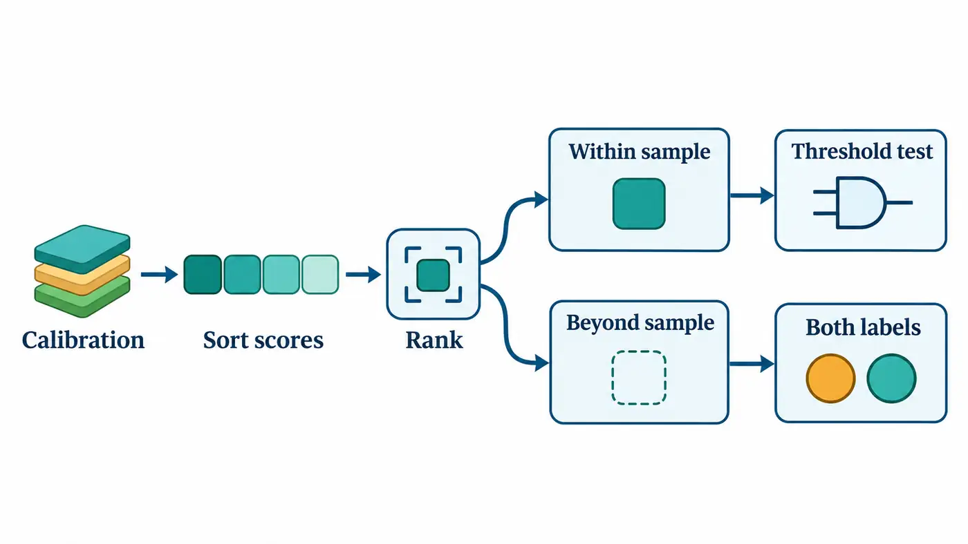
Continuing the segmentation of the previous article Conformal Prediction . Fix the trained classifier first, and write the "inappropriateness" between each possible answer and the input into the number of fractions. The LAC is used here, and the method is to subtract the probability of the model given to the label. When using labeled calibration data, only one score corresponding to the true label is handed over for each sentence. When predicting a new sentence, both negative and positive candidates can be examined at the same time, and those with a score below or equal to a threshold can be left.
here is to enter a movie review, is a candidate label, It is the probability that the output of the two-column model is normalized to this class after normalization. is the number of calibration sentences with true labels, is the allowable marginal leakage coverage probability, From the beginning of the number, the rounding symbol in the formula means the rounding up. The threshold is taken from small to large Calibration score; if this position exceeds the calibration table, set the threshold to positive infinity. This rule gives a clear result for any limited candidate score.
Why count one more position? Under the condition that the calibration sample and the next sample are exchangeable and the score rule has been fixed, it is conceivable to cover which one is new, and then sort all the true label scores together. When there is no parallel, the new sample has the same chance at each location. Retaining the equals sign when there is a parallel will accept the candidates on the boundary together. Covering the theorem is the probability of averaging the calibration and future samples together; holding the eight sentences that have been drawn, it is impossible to read a new film review from the theorem, Accuracy. The argument of the paper also does not use the observation frequency of these 360 film reviews.
Eight calibration scores plus a new score, a total of nine possible locations. Even if the largest score in the eight items is used as a threshold, in the ideal situation of continuous and exchangeable, it can only cover the first eight positions, and 8 is still lower than 90% by 9. In order to reach the target, the ninth position must also be included. There is no ninth value in the calibration table, and there are specific operating meanings here, and both candidates will be included in the collection. When it is changed to nine calibrations, there are ten positions in total, just cover the first nine, and you can do it with the maximum value of the nine. From this, it can be predicted when the threshold can be limited, but it cannot be predicted how much the set will shrink.
A minimal experiment and evaluation protocol
The last time the calibration scale was fixed, the sample division was changed, and the denominator covered multiple times was examined. In this order, you can only gradually relax how many calibration labels you can see. Use the SST-2 Validation identity list registered before the first project forecast of the project. There are 256 calibration pools, and there are 360 agreement audit pools, and the identities of the two have no intersection. The former retains the order of the original hashed. Each file is taken from the beginning, so the first file of the nine lines contains the eight and the one; this pairing makes which record is new between the two gears that can be traced back.
The scale of the pre-write protocol is 4, 8, 9, 10, 18, 19, 20, 32, 64, 128, 256. The nine tests can take the position of the limited threshold for the first time, and the nineteen tests change the position from taking the maximum value to the position that can skip a maximum value. Computing the standard rules side-by-side with a deliberate typo in each gear: When the rank crosses the line, the control cuts it to the last existing position. In this way, the two methods have the same input, budget and evaluation samples, and the difference can only be processed from the boundary. All gears are reserved, and the audit label is only used for counting.
Enter the DistilBERT checkpoint from the public English SST-2 emotion classification. Reuse the original two columns of logits saved in the 256 calibration records, that is, the output of the sort head before normalization. The audit side first did a CPU test run, and then used the same fixed model to re-tokenize and forward pass. There are up to 16 sentences in each batch, and the output shape is the batch of two. The maximum absolute difference between the two columns of the official replay and the archive is zero. The official batch tokenization is about 1.25 seconds with the forward loop, and the process peak memory is about 914 MiB. SST-2 has been used many times in the old round and this round, which is a method audit on historical data. IMDb is not read or added artificial semantic tags.
The coverage denominator includes every audit sentence. The numerator counts sentences whose returned set contains the original true label. We also count how many sentences receive zero, one, or two candidates and divide the total number of candidates by 360 to get mean set size. Sentences with empty sets count in both denominators. Measuring coverage only on sentences the model is willing to answer would condition the denominator on acceptance, making the result unsuitable for direct comparison with the conformal target.
What we tested
| Number of calibrations | target rank | Empty sets/single tags/double labels of standard rules | Number of coverage sentences (360 in total) |
|---|---|---|---|
| 4、8 | 5 and 9 respectively | 0/0/360 | 360 |
| 9、10 | 9 and 10 | 0/287/73 | 350 |
| 18 | 18 | 0/242/118 | 353 |
| 19、20 | 18 and 19 respectively | 0/287/73 | 350 |
| 32 | 30 | 0/335/25 | 339 |
| 64、128 | 59 and 117 respectively | 0/337/23 | 338 |
| 256 | 232 | 0/351/9 | 333 |
From eight to nine, the true class score of the new calibration sentence is about 0.993880, which became the maximum value at that time. After handing this threshold to the audit set, there are still two candidates of seventy-three sentences to pass together, and only one candidate has passed the remaining two hundred and eighty-seven sentences. Three hundred and fifty sentences of coverage mean that the correct answer is excluded from ten single tag sets. Starting with "double label all coverage", the profit of this change is to give more single answers, and the price can also accurately determine which ten sentences it is. The result given to Article 10 is the same as that of the nine, because the maximum value is still taken, and the new entry has not been refreshed.
There is a reverse change that is easy to misreport. From ten to eighteen, the average size has risen from about 1.203 to 1.328, and the double label has 45 more sentences, but only three more sentences are covered. Take the maximum value on both ends on this prefix, and add a new entry to push the maximum value higher. When the 19th article was added, the 18th elementary school became the penultimate position, and the threshold fell. This explains why the Calibration Set does not require the collection of each step to be smaller. It also puts forward a requirement for the comparison curve: it is the direct cause of the number of small points that are actually taken in each file, and how far the two scores are to be nearby, and the number of cursor samples will be omitted and changed.
With eight calibration examples, the rank-clipping comparison gave a sharply different result. The largest calibration score was only about 0.003028, so a candidate needed a probability of about 0.996972 or higher to qualify. Of the audit sentences, 91 got empty sets and 269 got a single label. The sets covered 261 sentences, or 72.5%. Mean set size was about 0.747, less than one candidate per sentence. A report that equated efficiency with small average sets would reward the worst undercoverage. At nine calibration examples, the two implementations agreed on every decision. Regression tests using only dozens or hundreds of calibration examples could miss this bug entirely.
Reading the official code and diagnosing failures
Starting with TorchCP's LAC scorer, first look for two fetching paths that provide labels and do not provide labels. Re-read the public function CALCULATE_CONFORMAL_VALUE: Check the relationship between the number of calibrations and the target rank, the cross-border branch directly returns to the positive infinite, and the rest of the cases call the order statistic function. Finally, the segmentation predictor is returned, and the tracking threshold is used to test candidates. The fixed versions and specific line numbers of these three places are in the source map. In this paper, the standard library is used to independently implement the rank and anthology, and the model forward directly calls the official classification of Transformers.
Three details are most likely to be confused when implemented. The sorted array is addressed from zero, and the mathematical ninth element is at the subscript eight. The probability direction should also be checked, and the higher true class probability corresponds to a smaller score. Finally, the default interpolation quantile may pick the number between the two observations, which both change the threshold and may cover up the border. This article writes one-tenth as an exact fraction to take an integer rank. In the log, the JSON null value is specially encoded for the infinite threshold, and the re-reading needs to be restored to the branch that accepts all the candidates; if it is regarded as a measurement missing and discarded, the two most important files will disappear from the result table.
Independent audit takes another calculation path. For two classifications, the inappropriateness of the candidates increases monotonically with "another type of output minus that type of output". For an audit candidate, there are several differences in the direct number calibration true class that are strictly smaller than it. If the count is less than the target rank, it is accepted, and if it is exactly the same, the candidate has already crossed that position. In this way, all collections can be reconstructed without calling the probability calculation, sorting and threshold functions of the main program. The script uses archived audit logits to check 22 conditions, 7,920 sets and 15,840 members to decide, and then calculate the size distribution and coverage. The evidence here is an executable arithmetic check, and the original emotion tag is taken from the dataset.
Code and instructions for reproducing the results
The fixed version has been made public, available from Source code directory enter, press Reproducing the results run, or control Where the equations appear in the official code Check the implementation.
Enter the source code directory of this article to execute:
python run.py
python audit.py
The first command reconstructs the result table, sentence-by-sentence collection and input summary with the real prediction of the package, and the second item outputs the independent verification result. If you want to check an endpoint, first locate the calibration scale and rules in the result table, and then use the same key to open the sentence-by-sline collection, and align the output according to the original sample identity. When the classifier needs to be rerun, the reproduction instructions give commands for fixed dependencies, caching, eight test runs and complete audits. Original movie reviews and model weights are obtained through respective public sources.
Research questions and summary
The authors infer that it can be split into two verifiable expectations. Keep 90% of the goals and the current non-random rules, change the calibration sequence, and still give two labels to all sentences in eight. This can be judged before running the model. The number of single labels at nine times depends on the maximum score of the new prefix and the score of the audit candidates, and there may not be 287 sentences after the order change. This experiment only runs a pre-registered nested path, and there is no repeated sampling error in the difference. If you want to estimate the fluctuation of the number of single labels after the change of the sequence, you should register multiple groups of sequences in advance and share the same batch of audit sentences; you cannot use the one transition here as a fluctuation range.
When you see apparently perfect coverage, ask whether every candidate was returned for every example. When the average set looks impressively small, check how many sets were empty and how often they left out the true class. The model supplied the same two columns of outputs throughout this comparison. What determined whether the sets could distinguish between candidates was whether the target rank fell within the calibration table and which scores lay near that rank. The next step is to apply the same rule to predefined subgroups and see what the overall coverage conceals.
References
The search date is 2026-11-14.
- Angelopoulos, Bates, "A Gentle Introduction to Conformal Prediction and Distribution-Free Uncertainty Quantification", 2021 First public in the year. See Section 1 of the structure and coverage theorem of the segmented conformity, and see the appendix for the rank demonstration under the limited sample. Full text from the authors
- SUSTech-ML, TorchCP, pinned version of the limited sample take rank and cross-border processing. Quantitative realization
- Hugging Face, English SST-2 classification header and label configuration. Pinned model revision
- Stanford NLP, SST-2, Validation division and data identity. Pinned dataset revision
Apps by the author
I also build small tools for everyday life. Here are two of my apps:
- Daily Expense Journal: Track your income and spending, plan a budget and set savings goals. View on the App Store.
- One Small Action: Pick a small action that fits the time and energy you have today, then record how it felt and what you noticed. View on the App Store.
Find more articles and projects on my website: zffjzz.top. I’d love to hear how the apps work for you and what I could improve.