The confidence lab: from model confidence to testing when to abstain

The same set of rules covered by 90% of the same set covers only 99/128 in one batch of film reviews, and 126/128 in another batch. The two batches use the same classifier, the same scoring method, and even from the same prediction document. Should I look up the code, or should I rewrite our understanding of "90%"? This time, separate the two: first verify each hit by the second program, and then ask who this percentage is established.
In the previous article, I made a calibration with a fixed list, and covered 333 articles in 360 audit film reviews. This gives a recalculable score, but doesn't tell us what to do with a calibration list. This article only changes the role of the sample. The average coverage rate of 200 internal divisions is 90.51%, in 82 times less than 90%. These two readings can be true at the same time. To understand them, you need to write what changes when sampling on the paper first.
Write "guaranteed" as an event first
Given a short review of the movie, the classifier gives positive and negative two-column scores. We allow rules to hand over a set of tags, such as only handing over the front, or both labels can be handed over. The reviewer has the true label provided by the dataset in his hand; as long as it is in the set, it is covered once. Therefore, a collection with two tags will inevitably hit, but it does not solve the problem of choosing one of the emotions. Whether the coverage rate is missed or not, how specific the answer is not to measure, and it is not the "proportion of being willing to answer" in the abstention experiment.
Segmentation Conformal Prediction The labeled sample is dedicated to determining the threshold. The model and scoring rules must be fixed in advance. set the input as , the candidate labels are , the class score of the model after normalization is . We use the simplest classification non-compliance: . The higher the score, the more inconsistent this label is with the model output. Give each calibration sample only the score of the true label, and then queue up from small to large:
here is the number of calibrations, is the allowable marginal leakage coverage, Numbered from the beginning, is the -th smallest score. At test time the rule compares candidate labels without access to the true label. The true label is needed only to evaluate coverage. Each calibration list contained 128 examples. Allowing a 10% miss rate and rounding up gave rank 117. Candidates tied at the threshold were included. A rank beyond the list length calls for an infinite threshold. That case did not arise here.
Guaranteed by the paper can be read like this. Put the calibration samples together with a re-drawn labeled sample, and if the swap their position does not change the joint distribution, they are said to have exchangeability. If there is no parallelism for true class scores, the ranking of new samples in this team score is possible. The probability that it falls within the allowable ranking is , about 90.7%. In general, when the equivalent terms are preserved, it is usually written as the lower bound:
in the subscript is a random calibration list, It is a random new sample and label, and the set changes with the list. Here, the probability of the two is taken at the same time, which is called marginal coverage. If the list is nailed to death, ask how much the threshold can cover for future people, and the conditions have changed; if you specify a certain sentence, a certain real category or a certain type of writing, the problem has changed again. The original inequality does not answer these conditions one by one.
Minimum experiment: two observation windows, sharing a threshold
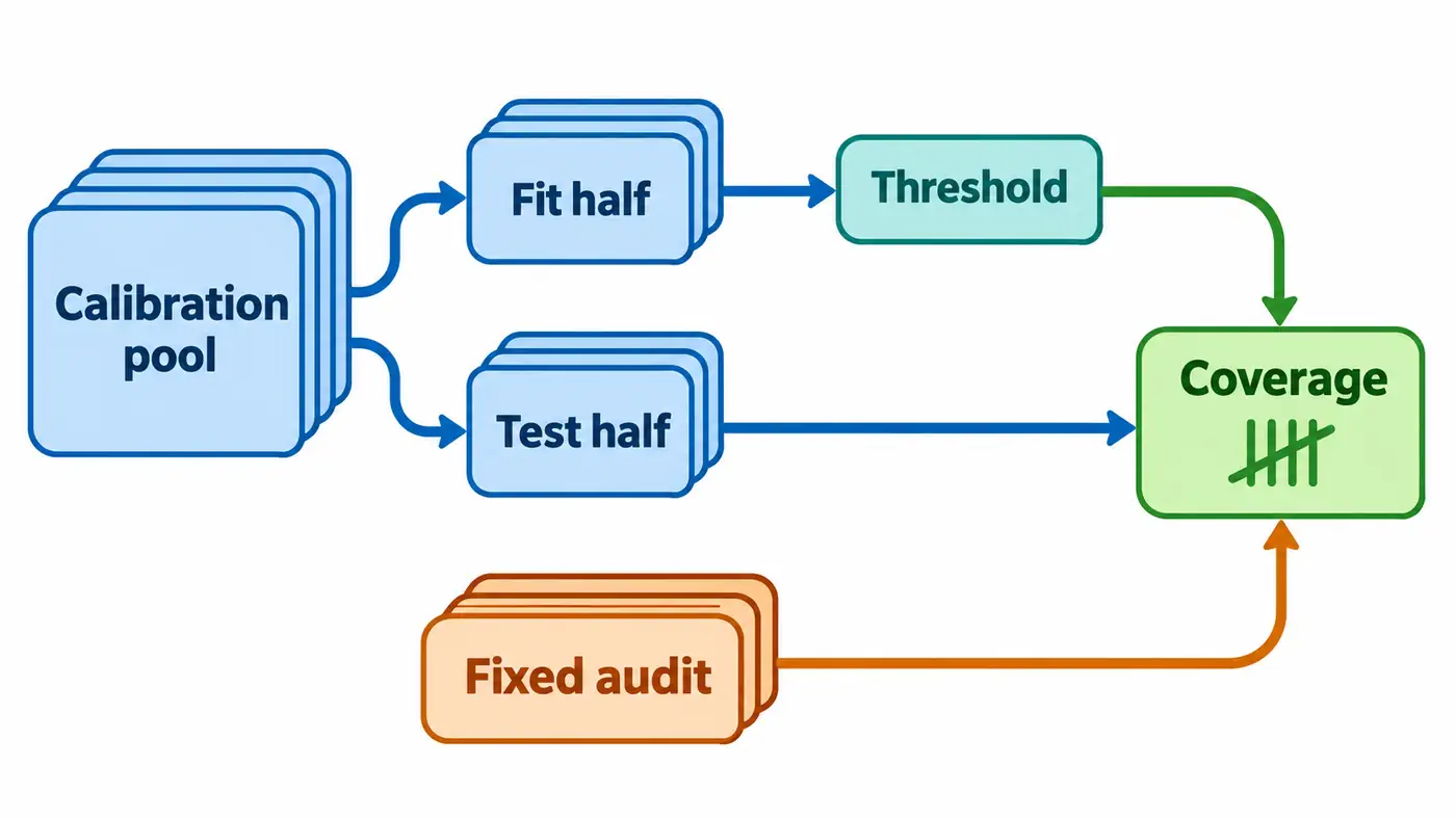
Take the public English SST-2 verification division and the Dissilbert header that has been Fine-Tuning. This data field was used in the early stages of the series, and the audit pool results have also been observed. Reshuffle will not make old materials the first blind test. We retain the three pools of exploration, calibration, and agreement audit previously registered, and only change the role in the original 256 calibration records. No external audit samples were put back to calibration, no read into the target domain IMDb, and no semantic labels were added.
Before looking at the results of this division, the agreement is fixed with two hundred seeds, from 12800 to 12999. Put together the decimal numbers of the seeds, colons, and samples, and sort them into a hash, sort them according to the abstract, the first half is fitted to the threshold, and the latter half is checked to cover. This is a pseudo-ran random replacement that is easy to recalculate; it is not stratified by true labels, and there is no result from multiple sets of seeds. Each pair of internal lists does not overlap each other, but different pairs use the same original sentences repeatedly. The fixed 360 audit samples are the second observation window. Each time, only the thresholds that have been calculated have been received, and they are counted separately, and they will never be combined with the internal results.
Two windows answer different questions. In the internal window, if the half-pool is fitted to a true label with a very low model score, the same record will be lost if the half pool is left; the composition and threshold of the list will change. In the fixed window, the evaluation object is always those 360, and any coverage changes can only come from the threshold changes. Comparing the two windows helps to locate fluctuations, but the difference between the mean value of the two columns cannot be regarded as an improvement brought by a certain method, because the denominator, specific sentence and sampling mechanism are different.
What really works and how to review the readings
Calibration pool multiplexed existing real model output. The audit pool starts with the locked public resources, first test runs in the central processor, and then re-run all 360 items according to the sixteen items in each batch. The model is in the evaluation mode, using a single precision, the upper limit of truncation is 512 tokens; each batch is output as a real number matrix with two rows by two. The official forward direction is about 1.30 seconds, and the peak memory of the process is 964,608,000 bytes. Compared with the historical audit output one by one, the maximum score difference between the official batch is zero. Two hundred times are divided into division of labor, there are no two hundred re-tokenization or retraining the model.
| Statistical caliber (200 times each) | average coverage | Minimum and maximum hit | Less than 90% of the division |
|---|---|---|---|
| Leave it in the same pool, 128 each time | 90.51% | 99–126 / 128 | 82 / 200 |
| Fixed audit, 360 each time | 92.04% | 304–343 / 360 | 33 / 200 |
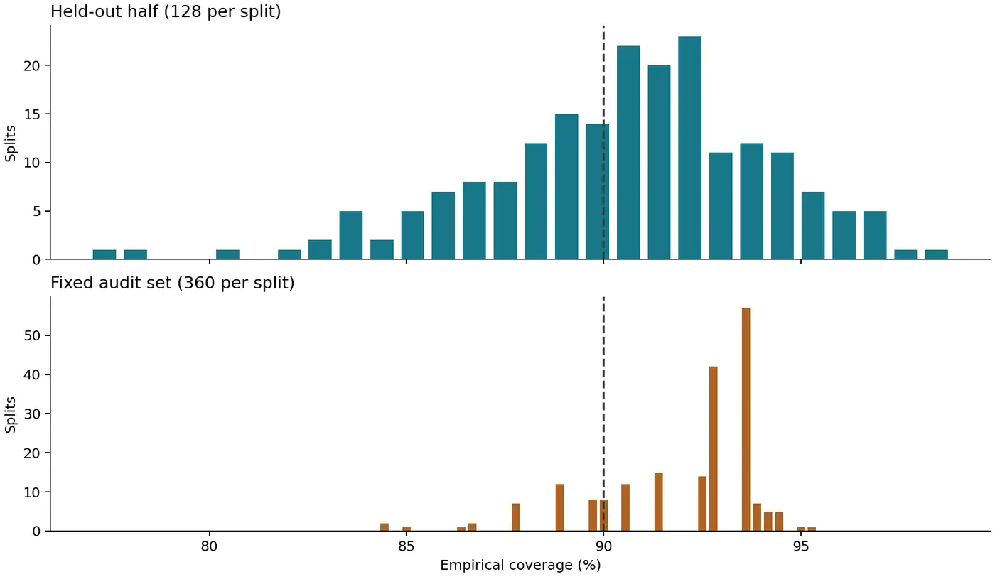
The horizontal axis is the actual number of hits divided by the current denominator; the vertical axis is the division number that produces this reading. Each picture is several times alone, and the vertical axis scale is also marked separately. The dashed line marks the nominal target, and there is no fitting smooth curve. In the first picture, one hundred and fifteen hits is still not enough, and it is not enough to cross the line until one hundred and sixteen. The second picture is exactly 324, which is 90%, and the statistics are not included when it is "lower than". Just rounding the printed percentages and comparing them may falsely report a boundary problem into an experimental abnormality.
You can check the origin of the form along the first log. The threshold for seed 12800 is about 0.93681, and 121 hits are left internally; 23 of the fixed audit are missed, and 337 are hit. The threshold value is large, and the allowable range is relaxed on the non-compliance axis, and it is not required that the classifier has more than 93% confidence. Add 23,171 to all internal hits, divide by 25,600 evaluation positions, and get the mean in the table. This denominator is the number of combined positions of "divided and sampled", and there are no 25,600 independent film reviews.
Read down the sample IDs instead. Across splits, each review was held out between 81 and 121 times. Of the 256 reviews, 218 were covered every time they were held out, 15 were never covered, and the other 23 changed with the threshold. The sentence and its official label stayed fixed. What varied was which other sentences made up the calibration set. For the 15 that were always missed, these counts describe only the thresholds we calculated. They do not imply a zero probability of coverage in the wider population. Writing “90% chance of protection” beside every review would erase differences we can check directly.
Guide to the official implementation and independent verification
When looking at TorchCP, you can skip the training interface first, and read from the two entrances of the classification scoringr: the corresponding column is given to the given label, and all columns are scored without the label. Then go to the public tool to find a finite sample rank, which calls the sequential statistic, instead of interpolation between two adjacent numbers. Finally, read the segmentation predictor and confirm the score direction of the comparison. On the model side, you only need to map the classification header and label map of the Transformers. After reading this route, you can distinguish which part is the existing collection rules and which part is the newly added duplicate division in this article.
Local analysis uses double-precision to restore the two types of probability, and the official independent recalculation will completely bypass this probability code: under the two classification, the larger the difference between the original score of the class subtracted and subtracted, the greater the non-conformity of the true class. Therefore, the second script can directly arrange the difference in scores, with the twelfth bottom as the threshold, and only the transformation is made when the value threshold is checked. The script rebuilds each pair of lists, compares two sets of uncovered numbers one by one, and finally compares the summary. In this way, even if the negative category column is wrongly taken, it is not easy to get confused in the two implementations at the same time.
Failure Troubleshooting: Distinguishing Arithmetic Errors and Research Errors
The first independent check flagged a discrepancy in the summary table. Every per-example inclusion decision matched. The mean for the fixed audit set differed in the last floating-point digit because one calculation averaged the hit counts before dividing by the denominator, while the other summed the integers before dividing once. The final implementation keeps integer numerators and denominators until it writes the result. On rerunning, all 200 thresholds, all 97,600 decisions about including the true class, and the counts by identifier matched. We kept the seeds, thresholds, and tolerance as specified and retained the splits that fell short of the target.
There is also an error that will not make the program report an error: Confidence interval on both ends of the figure as the overall coverage. The two ends are just the extreme value of this batch of data and the actual experience of this group of seeds. Increasing the seeds will show more arrangements of the same set of scores, but will not add a new review from the real world. In particular, the inner two halves complement each other, and the difficult cases are divided into which side will affect both sides at the same time. We neither use these hits as independent Bernoulli trials to draw an error line for the overall mean, nor interpret the 82 times below the line as a 41 percent chance of the theorem fails.
Research questions and summary
The author's explanation is: the average number of a fixed pool can be close to the nominal coverage, and at the same time, several fixed samples continue to be missed; "closer to the target" and "every object is also protected" is not the same assumption. To verify coverage on new sources, you need to pre-lock new sources, forecast configurations, and audit lists. If you want to test a certain type of short review, you must first define the category or length rule, and then report the denominator one by one. You can't find the worst ten of today and then give them a semantic name. Both of these are beyond the scope of the evidence for this redivision.
The next step can be verified to be smaller: keep the scoring device still, only reduce the length of the calibration list, record when the upward ranking is jumped, and whether the collection size also jumps. Today's experiments deliberately did not change the length, so the fluctuation can be put into the list and threshold, but there is no evidence to put it to the sample size. Keeping this difference is more useful than picking out a list that just covers 90%.
Code and instructions for reproducing the results
The fixed version has been made public, available from Source code directory enter, press Reproducing the results run, or control Where the equations appear in the official code Check the implementation.
Enter the source code directory to execute python run.py, can be divided into detailed, number-by-number counting and summary table from the real output of the package; python audit.py Can be reviewed independently. You need to redo the tokenization and at inference time, and follow the instructions to get the pinned version of the model and raw data. The source code does not distribute model weights or original sentences.
References
The search date is 2026-11-13.
- Angelopoulos, Bates, "A Gentle Introduction to Conformal Prediction and Distribution-Free Uncertainty Quantification", 2021 First public in the year. The structure and coverage of the division and conformity are shown in the first section, and the third section is repeated for the repeated division evaluation. Full text from the authors
- SUSTech-ML, TorchCP, pinned version of the classification scorer. LAC implementation
- Hugging Face, English SST-2 classification header and label configuration. Pinned model revision
- Stanford NLP, SST-2, Validation division and data identity. Pinned dataset revision
Apps by the author
I also build small tools for everyday life. Here are two of my apps:
- Daily Expense Journal: Track your income and spending, plan a budget and set savings goals. View on the App Store.
- One Small Action: Pick a small action that fits the time and energy you have today, then record how it felt and what you noticed. View on the App Store.
Find more articles and projects on my website: zffjzz.top. I’d love to hear how the apps work for you and what I could improve.