The confidence lab: from model confidence to testing when to abstain

On sample No. 230 of SST-2, the model gives the negative label about 0.6403, and the positive label is about 0.3597. When you can only submit one answer, it chooses a negative, but the official label is positive. If a set of labels is allowed in advance, is the second tag eligible to stay? No. 685 in the same batch of data was also misjudged as a negative side, but this time it only got about 0.0013. The two errors each occupy one grid in the Accuracy table, but there are different endings in the set prediction.
This article deals with these two examples with a pre-written rule, and also deals with all the remaining sentences of the same division. Models, texts, tags and reasoning budgets follow the previous chapter, changing the output form. After changing a single answer to a collection, the audit pool covers three more true tags. The price can be clearly pointed out from sentence to sentence: the nine sentences are given one more candidate, and the six sentences are already answered correctly.
Write the problem as a countable event
In the earlier abstention experiment, the coverage numerator counted sentences the model was willing to answer. Coverage means something different here. Each sentence gets a set, and even an empty set counts as one row in the denominator. We count the rows whose set contains the official label. This lets us evaluate both a classifier that gives a single answer and a rule that sometimes retains both positive and negative. Both outputs are checked against the same true-label column and use the same denominator.
Just staring at the coverage will encounter a very practical problem. If each line is filled with positive and negative, any answer from these two labels will be covered, but it will also lose the use of judgment emotions. Therefore, when registering the main indicators, we also registered the number and average size of empty sets, single-element sets, and complete sets. The control group directly takes the larger score of the same classification header, and each row has exactly one label. The two readings jointly answer a controlled question: how many candidates are returned after multiple selections are allowed, and how many errors are thus overwritten?
Scribing the ranking of true labels in the calibration pool
Fix a trained classifier first. The model outputs two un-normalized numbers for each sentence, called logits; doing softmax on the same row can get two column scores of sum in one. In order for each candidate to be compared with the same line, the definition of the candidate label is not consistent, that is, the degree that it does not match the current model judgment. Here is a simple fraction of LAC:
is a review, can be negative or positive, are the scores given by the classifier in this column. The larger the score, the harder the candidate to be retained. Each sentence of the calibration phase has an official label, so only check the column where the true label is located. The misjudged calibration samples are particularly worthy of retention, because the true class may fall just in a very low probability range. If you only collect the samples with the correct predictions, the group on which the threshold is based will change; if the total probability is to take the maximum probability, the column that needs to be observed is just jumped over.
To sort the true class of the calibration pool from small to large, select the threshold with a limited sample rank. Try two candidates separately when predicting, and all those who meet the target income set:
is the number of calibration sentences, is the probability of marginal leakage coverage allowed in advance, Refers to the first number from the beginning an observation. If this rank exceeds the number of calibration samples, the threshold is regarded as a positive infinity. This article is fixed , use 256 calibration samples, so the score of 232 small should be taken; one of the 231 items should be selected in the zero-based subscript of the procedure. The threshold obtained in this way comes from a real observation value, which is reserved when encountering equal candidates.
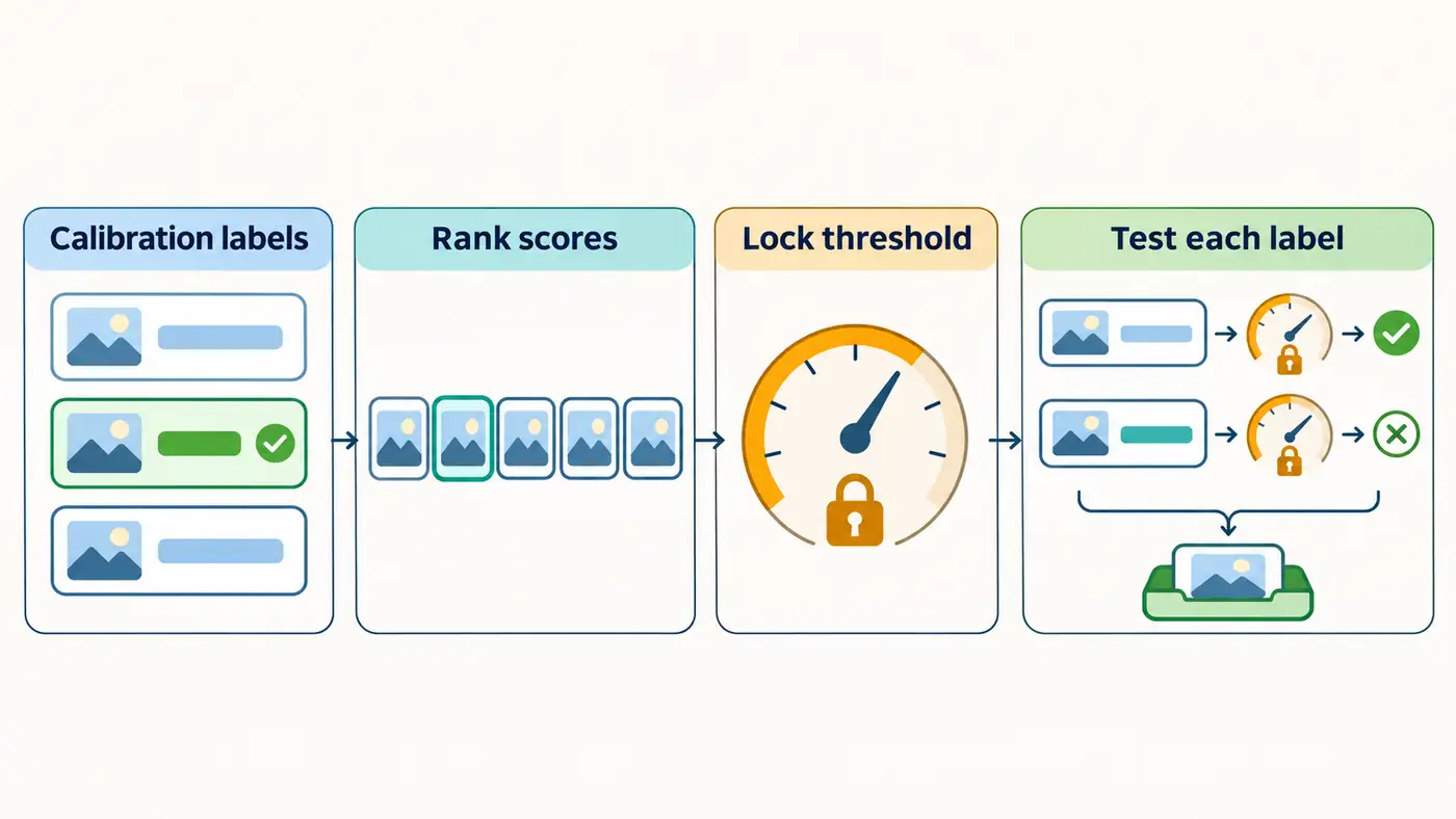
Why is one more multiplier? It is conceivable that the true class score of the next new sample is temporarily mixed into the calibration score, and there will be a total of 257 positions. If the scoring rules are fixed and these samples are interchangeable, that is, the swap order will not change the joint distribution, then the chances of the new sample falling on each rank will be the same when there is no parallelism. Leaving the highest prescribed number of locations to acceptable scores can control leakage coverage under the randomness of the Calibation Set and the new sample. Parallels may be more conservative when inclusions are processed. This argument does not require prior commitment that the probability scale of the classification header is already perfect.
A minimal experiment and evaluation protocol
The data comes from SST-2 validation of Stanford NLP. At the beginning of the series, three lists are registered according to the fixed hash order of the sample number. The first two hundred and fifty-six articles are used for early exploration, the next two hundred and fifty-six are for calibration, and the remaining three hundred and sixty are used for agreement auditing. Procedures check the identity, sequence, uniqueness and intersection of calibration and auditing. SST-2 has been used in historical research, and the performance of this batch of audit samples has also appeared before. This time, this is a method of reusing public data. IMDb development, calibration and final confirmation samples were not involved.
We used a pinned revision of the English DistilBERT SST-2 binary classifier, with label 0 for negative and 1 for positive. Calibration used the saved logits on their original scale, with the temperature transformation from the previous experiment removed. The calibration step wrote out the ranking and threshold before the analysis program opened the audit predictions. The protocol specified one target coverage level. The audit results played no part in choosing the score, target, or handling of empty sets. We needed no new semantic annotations: to check coverage, we simply looked for the dataset label in the returned set.
In the actual execution, first verify the cache weight, tokenizer and data file summary, and then use eight sentences on the CPU to test the run, and check the shape and label direction of the classification header. Formal reasoning to read all the audit sentences one by one, the upper limit of the batch is 16, and the maximum length is 512 tokens. The last dimension is always two categories, and the collection analysis is done after the row-by-line prediction is aligned with the original file. The official forward timer is about 1.38 seconds, the peak memory of the process is about 0.96 GB, and the timing does not include installation and weight downloads. Compared with archives, the maximum absolute difference of the official batch logits is zero.
What has the nine double-tag collections changed?
The measured nonconformity threshold is 0.718652, equivalent to a probability threshold of about 0.281348. Both candidates for example 230 clear the threshold, so the positive class stays in the set even though its probability is lower. Only the negative class clears it for example 685, preserving the model’s confident error. For example 527, the original negative prediction was correct at roughly 0.5354, yet the positive class at about 0.4646 also enters the set. That extra candidate adds no coverage.
| The same batch of 360 audit sentences | empty set | single element | double element | True class is covered | Average set size |
|---|---|---|---|---|---|
| Maximum order label | 0 | 360 | 0 | 330/360(91.67%) | 1.000 |
| Fixed threshold conformal set | 0 | 351 | 9 | 333/360(92.50%) | 1.025 |
Here you can do a cross-check without looking at the model name. The two probability is added as one, and the larger one is at least one-half. The calibrated probability line is less than one-half, so at least one candidate can pass the line per line, and the number of empty episodes must be zero. When both tags can pass, the complete works will appear, the nine complete works will each contribute two elements, and the rest will contribute one, with a total of three hundred and sixty-nine. Divide the total by 360 to get the average size in the table. If the program reports any empty sets at this time, the calculation should be checked first.
The nine complete works contain all possible official tags, and the remaining twenty-seven leaks occur in a single-element collection. Although this time, only 0.025 more tags are given to each sentence on average this time, the nine newly added candidates are not exchanged for error correction. Interpreting the coverage difference in the table as Accuracy increases will miss this cost: the reader still needs to decide how to use it after getting the dual-tag collection, and this experiment only checks whether the answer is in it. There is also no source of difficulty inferring the text of these nine sentences, and the score is close to the numerical relationship given by the model only.
You can also change a denominator to locate the table read error. Three hundred and fifty-one sentences are only given one label, and the collection of three hundred and twenty-four sentences includes the true category; add up these three hundred and twenty-four sentences and nine complete works to get the total number of coverages. If the research question is transferred back to "only answer when the only answer is given", the answer rate should be divided into 351 by 360, and the error rate in the answer should be calculated by dividing it by 351. These two items describe the additional quiz policy, which cannot be replaced with any of the experience coverage in the table.
Reading the official code and diagnosing failures
TorchCP can be read along the shape of the actual tensor. First look at how the LAC receives a batch of logits and how to normalize along the last dimension, and then look at how to index by row when the tag is passed in. After taking the true class, the calibration matrix is left with a number per row; when the label is not given, both columns are reserved. Next, read the common quantile function, check how it calculates the upward rounded rank, how to deal with the lack of samples, and finally go back to the Split Predictor, and see how it hand over the entire candidate fraction matrix to the collection generation function. This article is implemented using an independent standard library, and the source map is attached with the checked files and line numbers, which can be read step by step.
A common failure is to hand over the nine percentile directly to the default linear interpolation function. Even if the reader sees two realms that print out similar decimals, they should first compare the obtained rank, and then count how many candidates are between the two lines. Another error is to use the upper bound of non-compliance as the probability lower bound, and the code will still output a normal collection in form. Check No. 230 to distinguish between these two rules. Finally, check the denominator and evaluate the denominator; if you only score when giving a single-element answer, you will quietly switch to another selective classification experiment.
The independent recalculation script starts directly from the two columns of the archived logits, and calculates the difference value of the candidate column minus another column. Under the two-class softmax, the larger the difference, the higher the probability of the candidate. The scripts are sorted from large to small, and then compare the difference values on the selected positions one by one, bypass the index calculation and probability screening of the main program. The two paths are all consistent in the seven hundred and twenty-two candidate judgments, and at the same time check the sample identity, official label, collection size and single-label baseline. This is a reproducible arithmetic check that does not involve the emotion of re-evaluating any film reviews.
Research questions and summary
The paper’s marginal guarantee and the coverage measured for one batch involve different sources of randomness. The theorem considers the probability over fresh draws of calibration data and a new example. Here we fixed one threshold and counted hits on the same 360 sentences. We can report 92.50% as empirical coverage for this batch. Exceeding 90% once cannot establish exchangeability or promise at least 90% coverage for the next short review, for either sentiment class, or for long reviews in a different domain.
What is worth testing is that if the data source and scoring unit remain unchanged and only the calibration list is re-extracted, how much will the fluctuation of the threshold be transmitted to the audit coverage? This requires the number of re-divisions to be pre-specified and each result is preserved. The sorting, thresholds and set-by-sentence collections left today provide a checkable starting point. For this division, the most clear conclusion is that the model still has 30 single-label errors, the nine multiple-choices have only made up three of them, and the remaining 27 times can be positioned in the line-by-line record.
Code and instructions for reproducing the results
The fixed version has been made public, available from Source code directory enter, press Reproducing the results run, or control Where the equations appear in the official code Check the implementation.
Execute in the source directory python run.py, which can reconstruct the threshold, set and summary table from the attached real model output; then execute python audit.py Check the count. Readers who need to start with the original text can download the locking resources and replay the reasoning according to the instructions. The source code package provides only derived predictions and sample identities, and the original movie review and model weights are obtained from a fixed source.
References
The search date is 2026-11-12.
- Angelopoulos, Bates, "A Gentle Introduction to Conformal Prediction and Distribution-Free Uncertainty Quantification", 2021 First public in the year. See Section 1 of the structure and coverage theorem of the segmented conformity. Full text from the authors
- SUSTech-ML, TorchCP, pinned version of the classification scorer. LAC implementation
- Hugging Face, English SST-2 classification header and label configuration. Pinned model revision
- Stanford NLP, SST-2, Validation division and data identity. Pinned dataset revision
Apps by the author
I also build small tools for everyday life. Here are two of my apps:
- Daily Expense Journal: Track your income and spending, plan a budget and set savings goals. View on the App Store.
- One Small Action: Pick a small action that fits the time and energy you have today, then record how it felt and what you noticed. View on the App Store.
Find more articles and projects on my website: zffjzz.top. I’d love to hear how the apps work for you and what I could improve.