The confidence lab: from model confidence to testing when to abstain

The same sample, two seemingly contradictory results
In this audit, the short review number 382 was ranked 270th. The model originally gave 0.99695 points for its own answer, and only 0.91150 points after temperature scaling. If only the answer of Confidence reaches 0.99, this short comment will change from acceptance to abstention. If the model is asked to answer three-quarters of the question, it will be selected twice, and the last one will be selected both times. The data, answers and tags are all the same, how much has the abstention strategy changed?
This distinction is worth experimenting alone. In the previous article, in the calibration pool lock threshold, go to the audit pool to see how many errors it actually catches. This article puts the threshold aside, first gives the two groups of identical answer quotas, and checks who the quota is handed to. The research question is very narrow: for the same two-classifier, a global temperature learned from other samples, can you push a few more wrong sentences to the end of the queue? If it can, the reader should be able to point out the sample of the first exchange position.
What are the two readings measured?
Confidence is the probability of predicting the category. Calibration checks whether the value of the probability is commensurate with the long-term frequency. If a number of questions with different difficulty are grasped by 90%, you can observe the ratio of the actual answering of this batch of questions. If you disassemble a question separately, you can only see right or wrong once. Change a question, line up a stack of answer sheets, only take a part of the team's head, and hope that the fewer wrong questions will be the better. At this time, each score is written more conservatively, and it may not change the order of the team.
Guo, Pleiss, Sun, and Weinberger report in the calibration study of modern neural networks, and then fit a single temperature after training, which can improve the probability estimates of the multiple networks they test. This article borrows its transformation form to measure two specific readings on the archived emotion classifier. Negative log-likelihood takes the negative logarithm of the probability of the real class probability of each sample, and the more confident the model is wrong, the greater the cost. Another reading is the binning estimate of the Expected Calibration Error: the probability axis is divided into ten boxes, each box is compared with the actual accuracy, and the absolute value of the difference is taken and weighted according to the number of people in the box. The empty box contribution is zero. The nature of the two is different, and this article reports together according to the preset caliber.
Selective classification is an acceptance rule for the model. According to the definitions of Geifman and El-Yaniv, the coverage rate is the ratio accepted in all the samples to be answered, and the selectivity risk is the loss calculated on the accepted sample. This article uses the wrong one to record a loss, which is the conditional error rate. When only one question is connected, the wrong one is 100% of the risk; all rejects are zero. Leave the latter situation blank when drawing, so that you will not draw a perfect result at all.
Why two classifications can predict the entire curve
The categorical header outputs two unnormalized real numbers to each sentence, called logits. Use the difference between the two numbers to indicate which side the evidence is biased, and then use the temperature to adjust the relative strength of the two sides. Take the category with high probability, its Confidence can be written as
here is the sample number, and are negative and positive, respectively. is a difference without direction, is the positive temperature shared by all samples. Dividing both items by positive numbers will not swap their size, and the predicted labels will remain. More importantly, if A's difference is greater than B, after dividing the two by the same positive number, A's point difference is still larger. Substitute into the above formula, A's Confidence is still larger. When the difference between the two points is exactly the same, the two temperatures are tied; this experiment agrees that the tie shall be ascended according to the sample number.
From this relationship to Abstention, there is only one step away. For any given number of places, the same long prefix is intercepted for the original queue and the new queue. The two paragraphs contain the same identity, and the prediction category of each identity has not changed. The total number of errors is the same when compared to the official label. This reasoning holds even if a prefix does not happen to be wrong. It predicts the consistency of all places, and checking a good-looking point or comparing the average of the two curves is not enough to replace this test.
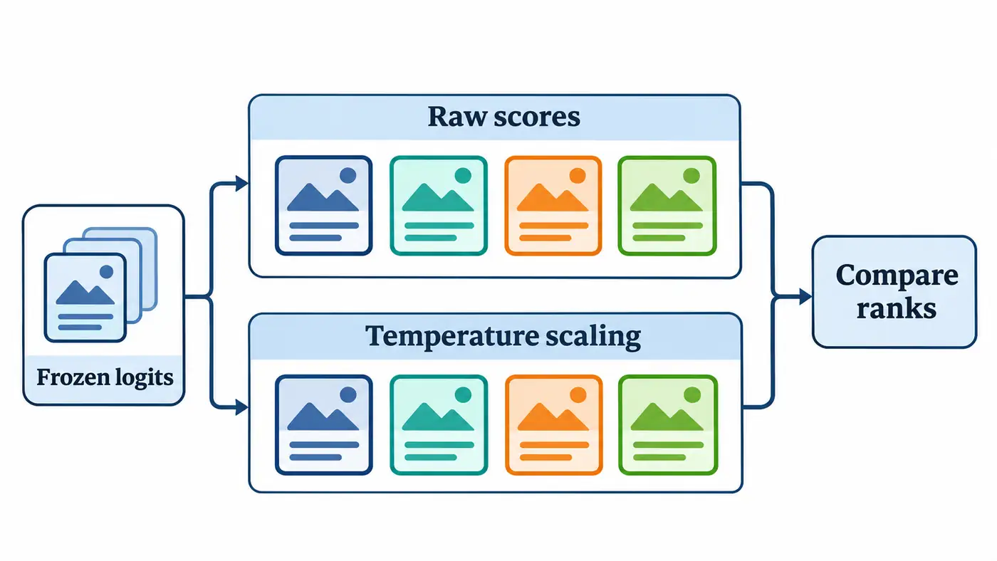
Data Registration and Minimum Experiment
The input is a pinned version of the DistilBERT English SST-2 emotional classification checkpoint, the category zero is negative, one is positive. At the beginning of the series, the Validation Set has been registered in the hash sequence of the sample identity, the first 256 articles are used for exploration, and then 256 articles are used for calibration, and the remaining 360 articles are used for agreement auditing. The entire Validation Set has been touched in the history series, and the audit pool has also been observed before. These data are suitable for verifying a clear mathematical prophecy, and cannot assume the role of independently confirming a new discovery. This time, there is no visit to IMDb, and there is no new label that needs to be judged by real people.
Pre-lock two sets of temperatures: take one of the original group, and the scaling group directly reads the 2.481924 obtained by the previous calibration pool to minimize the average negative log-likelihood. Audit labels are only used when judging whether the answer is correct or not and the calculation of the loss. The program checks the calibration prediction hash of the two pools of identity mutually exclusive and in the temperature file, and recalculates the objective function gradient at the inverse temperature from the calibration sample. This can distinguish "read the same parameter file" and "the value in this file is in line with this batch of calibration data". There is no search for the temperature that makes the audit curve the best.
The real model first replays eight sentences in the central processing unit, checks the label mapping, tensor shape, limited output and resource occupation, and then replays all the audit samples according to sixteen sentences in each batch. Fixed four threads, single precision, evaluation mode and the upper truncation limit of five hundred and twelve tokens, using the same vocabulary and model weights. The number of columns output by each batch header must be two; the last batch has only eight rows, counted according to the actual row count. Forward and sorting of the official batch takes about 1.29 seconds, the peak memory of the process is about 899 MiB. The timing here starts after the model is loaded and cannot be regarded as the total time-consuming of the first download and startup.
Measured results: align the quota first, then look at the threshold
| audit indicators | original fraction | After temperature scaling |
|---|---|---|
| Average Negative Log-Likelihood | 0.38411 | 0.23714 |
| Ten-box calibration error | 0.07327 | 0.01990 |
| Errors when 270 are fixedly accepted | 8 | 8 |
| Average risk for all non-null prefixes | 0.02124 | 0.02124 |
| Acceptance at fixed 0.99 threshold | 304 | 0 |
There is no exchange in one of these 360 positions, and neither group is equally divided. Check all non-null prefixes one by one, and the cumulative errors are the same everywhere. All thirty are wrong, and three-quarters are covered by eight. The denominator of the latter result is 270, corresponding to about 2.96%. It also tells us that there are twenty-two mistakes in the ninety articles left at the end of the line. The calibrated team retained this screening ability and also retained the eight mistakes in the front.
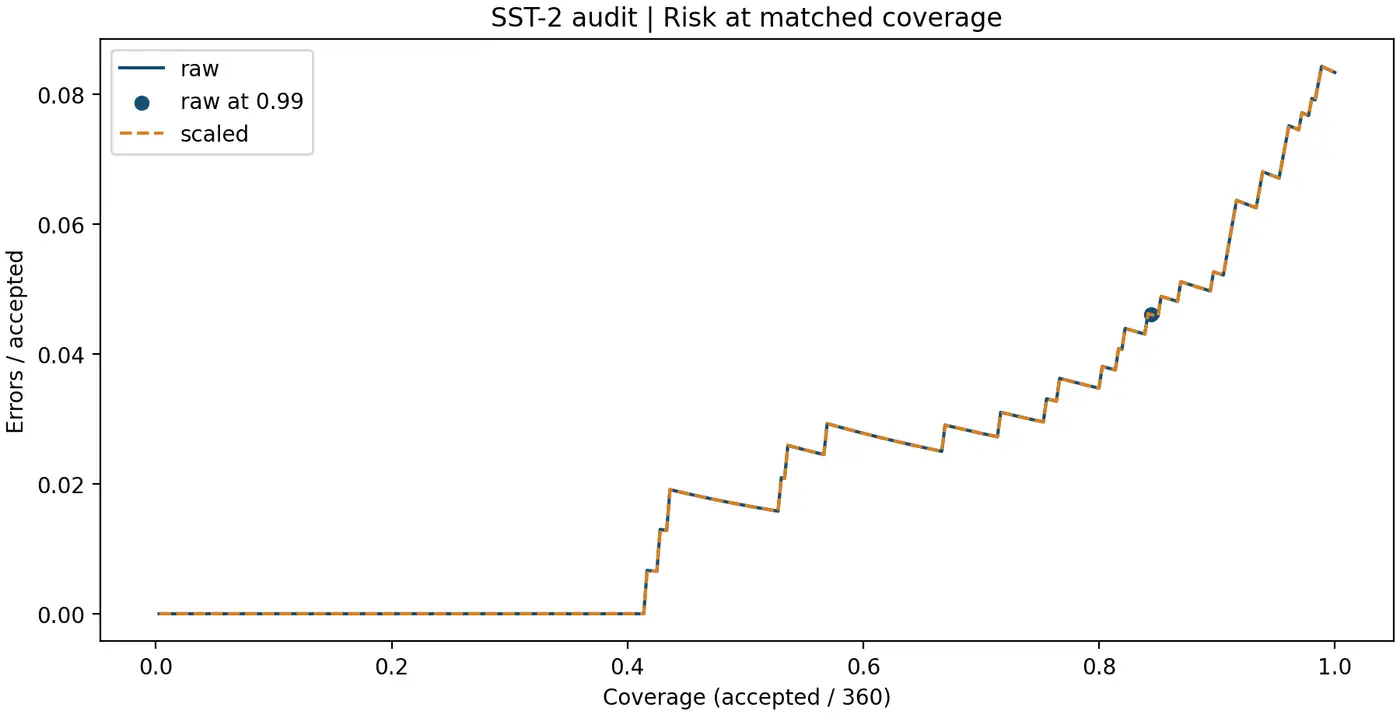
The horizontal axis in the figure is the answer ratio, and the vertical axis is the ratio of the wrong questions of the answered part. The solid blue lines and orange dotted lines are stacked on the same trajectory. The position of the original group of 0.99 is marked with points; the top sample of the scaling group is only 0.97551, and no one has reached this line, so there is no risk point to draw. The fourteen errors under the original threshold are divided by 304 and about 4.61%. Compare it directly with the zero acceptance errors of the scale group, which will quietly lose the denominator and get an unfulfilled improvement.
In this actual verification, the lower Negative Log-likelihood shows that the logarithmic probability obtained by the real category has increased on average; the smaller ten-box error shows that the frequency under the box is closer to Confidence. These two sentences only talk about the summary of the whole sample. Going back to the correct short comment at the beginning, lowering the correct answer will make its own negative log-likelihood rise. The overall improvement can be accompanied by deterioration of individuals, just as the average risk is not enough to prove the ranking of each sample alone. Sampling records allow both inferences to be checked directly.
Reading the official code and diagnosing failures
Read the forward function of the official classification head first, and see how the first tokens pass through the linear layer, the activation, discard layer and the last classification layer. Re-read the temperature scaling function implemented by the author of the calibration paper, which extends the temperature to the shape that is compatible with the output, and then divides the elements one by one. Finally, look at the local evaluation script: subtract the maximum value from each row and operate with a stable index, normalize to obtain two types of probability, and sort by the maximum probability of not rounding. This sequence can prevent the maximum raw output from being mistakenly regarded as Confidence . Adding the same constant to the two original outputs of a sentence at the same time, the probability remains unchanged, but the maximum original output will change.
If the ranking changes, first find the identity of the two queues for the first time, and print the original difference between the two lines and the saved fractions to enough decimal places. Leaving only two decimals makes many of the probabilities close to one look equal, and then you may change the order by breaking the identity. Further check whether it is converted to low precision after scaling, or the two groups use different tokenization upper limits. The former will create a numerical tie, and the latter will change the original input evidence. Both can be another interesting experiment, but it cannot be used to overthrow the derivation of the shared real-number transformation.
The absolute difference between the eight-sentence test run and the archive output is about , the official batch is the same as the archive by value. The numerical deviation of the small batch is recorded in the environment file, and the prediction category, identity and text abstract are also checked one by one during the acceptance. Independent re-calculation is switched to high-precision decimal operation, and Confidence is directly found from the absolute difference. The original sentence is not distributed with the package, and the downloader will check the data file and weights one by one.
Research questions and summary
Two extensions would be worth testing. First, what if each example has its own temperature? Of two nearly equal score gaps, the larger one could fall behind if divided by a larger temperature. Second, what happens with three or more classes? The top class’s probability then depends on the scores of all competing classes. The gap between first and second alone cannot reconstruct the denominator. These hypotheses follow from the limits of the derivation. We did not run either condition or use the audit pool to choose an alternative.
If you want to reuse an old threshold, try this with pencil and paper. Convert the old probability cutoff to the minimum raw score gap it requires, then convert that gap back to a probability using the new temperature. With ideal numerical precision, this preserves the accepted set. It preserves the decisions only: a new sample distribution can still change the risk among accepted cases. When reading the results, first ask what the horizontal axis holds fixed, then whether the accepted set changed, and only then interpret the change in probability quality. The conclusion here depends on using the same binary classifier, a shared positive temperature, and a comparison at equal coverage.
Code and instructions for reproducing the results
The fixed version has been made public, available from Source code directory enter, press Reproducing the results run, or control Where the equations appear in the official code Check the implementation.
Execute in this source code directory python run.py, you can regenerate the sample-by-sample double-column score, all prefixes and sum of indicators from the fixed prediction; then execute python audit.py Take the independent recalculation path. To start replaying from the weight, prepare official resources according to the instructions, and then perform the eight-sentence test run and the official operation of the 360 sentences. Both paths have been executed this time, and the cache that has been verified one by one is reused in the download stage.
References
The search and version check date is 2026-11-11.
- Guo et al., on Calibration of Modern Neural Networks, ICML 2017
- DistilBERT SST-2 official model card and fixed version
- Stanford NLP, SST-2 dataset fixed version
- Hugging Face Transformers v4.49.0, Distinbert Category Header
- Geifman and El-Yaniv, Selective Classification for Deep Neural Networks, NeurIPS 2017
Apps by the author
I also build small tools for everyday life. Here are two of my apps:
- Daily Expense Journal: Track your income and spending, plan a budget and set savings goals. View on the App Store.
- One Small Action: Pick a small action that fits the time and energy you have today, then record how it felt and what you noticed. View on the App Store.
Find more articles and projects on my website: zffjzz.top. I’d love to hear how the apps work for you and what I could improve.