For graduate students, new research and engineering researchers; search and experiment date: 2026-09-15.

Abstract
A world model can generate plausible video and still predict the wrong future for a given action. We study this in a controlled oscillator. The models learn to predict the next state from trajectories, then predict forty steps ahead. We compare supplying the true state, feeding back the model’s predicted state, and periodically correcting it with observations. We ran nine small models across three data seeds, saved every set of weights and predictions, and independently recomputed the results. The experiment examines sequence prediction and its evaluation. It does not reproduce the racing or Minecraft settings, or the control results reported in the paper.
Contents
- Reproduce value: replace "like real" with a testable target
- Core ideas and formulas
- A guide to the official implementation
- A minimal experiment and its results
- Evaluation protocol and independent audit
- Troubleshooting and limits of the evidence
- Questions for further research
- Summary and References
Reproduce value: replace "like real" with a testable target
The world model learns how the environment changes with the action. The Rollout here refers to the continuous development of the future state from a starting point: the second step starts, and the input comes from the previous round of the model prediction. It is more likely to expose cumulative deviations than a single step review that gets the real state at each step. The advantage is that without the need to fully train the agent, you can first check whether the dynamic part is trusted.
Paper report: HA and Schmidhuber's World Models separate visual compression, time memory and controller; the memory module predicts the next latent variable distribution after a given action and historical information. The latent variable is the numerical representation of the compressed observation, which is not equal to the real physical state. The original method uses a mixed-density cyclic network to express a variety of possible futures, and the deterministic regression in this paper only retains the action condition to predict this interface. author interactive paper
DreamerV3 rolls out imagined trajectories in its learned latent dynamics and uses signals such as predicted rewards to learn behavior. We consulted the second version of the preprint, revised in 2024 and still titled Mastering Diverse Domains through World Models. This account is confined to that version and excludes material from the later journal article. Version page; Full text
This time, three distinguishable questions are raised: just look at what will be lost at the current location? How does the linear approximation fail after leaving the training range? How many errors can be relieved by reading the real state every few steps? The three questions change the state information, the function form and the observation budget respectively, and cannot be combined into a "model stronger" conclusion.
Core ideas and formulas
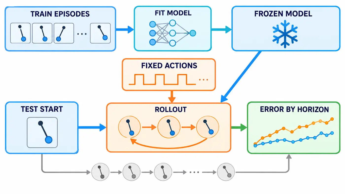
The top of the method diagram indicates the freeze model after training, and the lower part represents the test. The gray branch represents the truth value previously recorded under the same action sequence, and only enters the scorer; the curve and swing icon in the figure are both concepts, not measured curves. The actual learner is a small regressor, not a neural network implied by icons.
Constructing noise-free discrete systems:
is the dimensionless position coordinates, for the velocity variable, Sampling from the three values of negative half, zero and positive half. Status It is a two-dimensional vector, and the action is a one-dimensional scalar. It is a teaching oscillator with damping and external force, and the real device is not calibrated; the cover is not a measurement photo. Update the speed first, then update the position, and the exchange order will get different tracks.
All three learners use the least squares:
is the row eigenvector, stack training transfer, Save the corresponding next state, It is the coefficient to be learned; the square norm sums the residuals of the two outputs. The characteristics of the complete linear model are position, speed, action and constant, and the shape of the training matrix is , the goal is , the weight is .
The position model removes the speed, still predicts two outputs, a total of six parameters, but the next step does not use the predicted speed. The structural feature model adds a sine term after the complete linear feature, a total of ten parameters, which just covers the functional form of the real equation. This is the diagnostic reference of the known structure, and cannot be regarded as the automatic discovery of physical laws from the data.
During training, the input of each transfer is a true value, which corresponds to the teacher forcing, that is, the real previous step is used as the prediction condition. open development , only set at the starting point . Subsequent real states can be used to calculate errors, but cannot enter the predictor; the action must also be consistent with the generation of truth values.
A guide to the official implementation
Read the original repository first rnn_train.py. Location random_batch, it samples the latent variable from the encoded mean and variance; then inputs the current latent variable and action, and then outputs the slice that takes the wrong sequence of the latent variable back. Draw this alignment relationship first, and then look at the optimizer, you can find the problem of mismatching the action to the next frame as soon as possible.
Then read rnn.py: The input width 35 comes from 32-dimensional latent variables and three action channels; the mixed head output weight, mean and log standard deviation, and calculate the negative log-likelihood by logarithmic summation. Again sample_sequence See how the generated value is written back prev_x, how to update the loop status. The source code uses the old TensorFlow interface, this time only read, and the compatibility is manually verified.
in DreamerV3 rssm.py , RSSM is a cyclic state space model. Compare observe and imagine: The former fuses the observation code, and the latter generates a priori from the internal state and action, and samples the next random state. Both of them are advancing, the difference is whether they have received observational evidence.
Final reading agent.py of report. The open forecast report first observes the first half of the sequence, and then uses the second half of the action to expand. The predictions here are conditional predictions for a given action. in the source code prevact Using the action caliber to reach the current observation, the time index should be checked when transplanting, and this article cannot be directly applied to this article. name.
The above branches are search days master or main, there is no pinned commit hash, and there is no guarantee that the paper version corresponds line by line. This NumPy script independently implements the teaching system, and there is no official encoder, random submersible state, reward head or strategy training.
A minimal experiment and its results
Run in the article directory, dependencies and complete instructions are available README:
python3 -m pip install -r code/requirements.txt
python3 code/world_model.py
python3 code/audit_results.py
The actual environment is Python 3.12.14, NumPy 2.3.5, and CPU double-precision. The three seeds generated 128 pieces of training, 32 development articles for development, and 64 trajectories for the same distribution test and 64 trajectories outside the distribution test, each forty transfers. Seed control data sampling, the least squares is not initialized randomly; the development set only records the indicators, and does not adjust the parameters according to this or select the model.
The initial position of the training, development and the same distribution test is between plus and minus 0.5; the out-of-distribution test is changed to 1.5-2.5. The initial speed is between positive and negative 0.3, and the action rules remain unchanged. The "same distribution" here describes the initial conditions and acquisition rules, and does not guarantee that the predicted state will always fall in the training trajectory coverage interval.
The following table is the mean of the three seeds, all use the position mean square error, and the seed results are different from the sample standard deviation. Complete summary. Forty input time on the single-step column is an average of forty input moments, and the last three columns are the designated steps that freely expand from a common starting point, and the sampling caliber of the two is different.
| Model and test conditions | single step error | Step 10 Error | 20th step error | 40th step error |
|---|---|---|---|---|
| location only, same distribution | 4.28e-4 | 0.0255 | 0.1112 | 0.1024 |
| complete linearity, same distribution | 9.31e-10 | 1.68e-6 | 6.32e-6 | 1.63e-5 |
| complete linear, out of distribution | 3.08e-5 | 0.2440 | 1.0553 | 0.0821 |
| sine structure, out of distribution | <1e-20 | <1e-20 | <1e-20 | <1e-20 |
What we tested: the complete linear model is more accurate near the training, but there is a significant deviation in the twentieth step outside the distribution; the 40th step is reduced, reminding us that the oscillation trajectory may be re-approached, and the end point error cannot represent the whole process. Only the position model is also failed in the same distribution test, indicating that the missing and distribution changes of the predicted condition are different problems.
The error of the structural model is close to the floating-point rounding level, because the feature covers the noise-free generation equation; the independent inspection also confirms that the learned coefficients are consistent with the equation. This result only proves that data, solution and unfolding can be aligned, not that the world model has solved the generalization problem.
Additional diagnostics reset the input to the real state every five steps. The full position error of the complete linear model outside the distribution has dropped from 0.46198 to 0.002255. The reset occurs before the next step is predicted, the rating still retains the previous error output, and the rating point is not forcibly changed to the true value. It adds a real-observation budget, not a model upgrade after retraining. operation record
Evaluation protocol and independent audit
The data is divided according to the complete trajectory, and the adjacent windows in the same round are prohibited from randomly assigned to training and testing. All models share the initial state and action under the same sub-subject, and the weight is only solved by the training transfer; the number of parameters is different, so the position ablation is not equal parameter control. Report the gradual error of position and speed, the text only selects the position for clear comparison, and cannot be ranked after arbitrarily mixing the two units.
Formal indicators are defined as
is the number of trajectories of the test condition, is the predicted step from the starting point, and Use the same action sequence. The whole process error is then averaged for forty steps; it is not the 40th step error. The standard deviation of the three data seeds reflects this set of sampling changes, which are not Confidence intervals, nor can the time in a trajectory be regarded as a separate sample.
independent audit If the training script is not imported, 34,560 real transfers, 172,800 prediction states, 172,800 prediction states, and 4,512 index values will be recalculated with scalar operations; the maximum prediction difference is about 4.0e-15. It also checks the initial state unique, structural coefficients, training matrix full rank and least squares residual conditions. Audit output
The inspection to prevent truth leakage is especially direct: all the states of the test trajectory other than the starting point are replaced with meaningless values, and the open prediction must be completely unchanged; the first step of the open prediction must also be equal to the single-step prediction of the same starting point. Both are passed. The saved array is enough for the reader to recalculate the table without trusting the body description.
Troubleshooting and limits of the evidence
First ask whether the observed state contains enough information. At zero position and zero action, velocities of +0.3 and −0.3 produce next positions that differ by 0.0588. The position-only model sees identical inputs for two different targets. More examples of the same kind cannot supply the missing information. A history of positions or an estimate of velocity could address the problem.
Check the function form and scope. The author infers that the training of the nearby sine function is approximately linear, which can explain the small single-step error of the complete linear model; the large initial position exposes this approximate deviation, and repeated re-irrigation changes the subsequent input. Structural reference supports this explanation, but this experiment did not decompose the local approximation error, state offset and the amplification effect of each step item by item.
Also, don't misread "error accumulation" as a necessary exponential explosion. The system has a damping, and the error can fluctuate; there is no unified growth rate. If you draw a picture, you should show the whole process and a clear vertical axis, and you cannot replace the step-by-step statistics with the two best-looking last frames.
There is no perceived noise, unpredictable event, action strategy change or learning controller in this experiment. Reading the full true state is ideal for every five steps to read the true sensor; the deterministic mean square error cannot measure whether the random predicted distribution is calibrated. Real images, official training, multistep learning goals and control return experiments are not run, and wait for manual verification.
Questions for further research
First, add two frame history to the position model, can the speed information be restored? Fixed the observation budget, compared the historical difference and the implicit state of learning, and added measurement noise to check whether the income depends on precise coordinates.
Second, does multistep loss training improve long-range prediction? Pre-determine the training steps and development selection rules, and report both single-step and long-range errors on the new Test Set at the same time, to avoid only showing favorable indicators after sacrificing local precision.
Third, when should it be corrected under the limited observation budget? Compare the fixed interval and the uncertainty trigger, the fixed number of readings, and then check the error peak. If the strategy is further learned, the rewards must be verified in the real simulator to prevent the strategy from using model errors to obtain false rewards.
Summary
The key to the experiment of the smallest world model is to clarify what the predictor can read at each step, and put the error back to the time axis. First distinguish the cost of status missing, approximate deviation and observation correction, and then discuss more complex latent variables and control learning, and the reproduction of the paper has the basis for gradually expanding.
References
The following links are actually retrieved and opened on 2026-09-15;
- David Ha、Jürgen Schmidhuber,2018, World Models,arXiv v1. Version page; author interactive paper. Continuous maintenance of the interactive page is not considered a verbatim snapshot of V1.
- The author's official experiment code, WorldModelsExperiments, the search day master. training slices; Hybrid Density Network and Sampling.
- Danijar Hafner、Jurgis Pasukonis、Jimmy Ba、Timothy Lillicrap,2023, Mastering Diverse Domains through World Models, 2024 revision v2. Version page; Full text.
- DreamerV3 official code, search the day main. cyclic state space model; Training and Open Forecast Report.