
Reproduce the goal: keep the accuracy as it is
In the previous fixed model prediction, only the binning method was changed, and it was found that the calibration error will change with the measurement caliber. This time, move forward further: If the prediction category of each sample is completely unchanged, should the quality of probability remain the same? This is not a word game. Accuracy only records whether the answer hits the label, can't distinguish a prudent error and a one that has little room for the correct answer. If the scientific research report only keeps one accuracy number, it may throw away all the differences.
This article has added a controlled control: fixed the existing real classification score, use the same positive temperature for all samples, and then compare the Negative log-likelihood and the briel score. The former is usually abbreviated as NLL, which measures the probability that the model assigns the real label; the latter is usually written as Brier, measuring how far the probability vector is from the real label vector. The lower the two the better. We don't train the model, we don't fit the parameters, and we don't choose a temperature from the results to bring it to the subsequent evaluation.
The conclusion of this actual verification is very specific: the four conditions are all 233 of the 256 articles are correct, but the probability loss is obviously different. This counterexample is enough to deny that "the same accuracy means the same quality of probability", but it is not enough to prove that a certain temperature must be better on new data.
Core idea: only change the sharpness of probability
The logits of the model output are class scores that have not yet been normalized. For each input, the classification header generates two numbers; the maximum score corresponds to the predicted category. The temperature transformation first divides these two numbers by a positive number at the same time, and then converts it to one by means of the probability:
here is the sample serial number, and is a category index, is the shape fixed fraction matrix, is the global temperature. The temperature of less than one usually makes the probability more sharp, and greater than one makes it tend to be uniform. Because dividing by the same positive number does not reverse the magnitude relationship, the maximum value position of each row remains unchanged under precise arithmetic. The original equal scores are still equal, so the rules of the draw should also be fixed.
Guo et al. studied temperature scaling in a 2017 paper and reported its calibration performance on the task of the study. The transformation form is borrowed here; the author implements the validation set to optimize the temperature, and this article does not perform that step. Readers should separate the "Fitting Methods of the Paper Report" and "The Measurement and Control of the Designated Temperature This Time" separately.
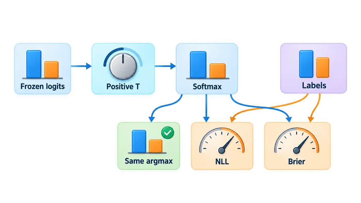
The label in the figure only enters the loss calculation and does not enter the temperature setting. The icon is a flow diagram, and the column and pointer have no numerical meaning; the real measurement results are shown in the following log drawing.
Formulas and modules: where is the probability wrong
Negative log-likelihood adopts natural logarithm, which is defined as:
for the total number of samples, for the official two-class label, to give the probability of the real category. Losses increase rapidly when the real class probability is close to zero. This makes a small amount of self-confidence errors likely to have a big impact on the total loss. The actual calculation adopts a stable logarithmic sum exponential form, and the loss is directly obtained from Logits, to avoid the logarithm of zero first and then the logarithm.
The Brier in this article uses the form of the two categories of square errors added:
Indicates that the function is one in the real class, and the rest is zero. The definition range is zero to two; if you only calculate the square difference of the positive-class probability and the zero one label, you will get half of the value of this article. Definitions are not equal to implementation errors, but cannot be directly compared without conversions. Independent auditing uses this double relationship under the two categories to prevent the main program from copying the same paragraph of sum logic as the check program.
Accuracy, log loss and squared loss answer different questions. The former ignores the probability change outside the maximum value; the latter two focus on the entire predictive distribution. This article does not equate the loss of probability loss with each Confidence interval calibrated, nor does it equate it with the improvement of Abstention sorting. The evaluation objects are different and require different experimental support.
A guide to the official implementation
First read the DistilBERT header in the pinned commit, and confirm that the hidden state of the first position has passed the pre-classification layer, activation and classifier to output two scores. Reread the label mapping in the model configuration: zero is negative, one is positive. Finally read the author repository of temperature scaling temperature_scale, it is confirmed that the temperature is divided by the logits, not the probability that it has been normalized. Direct division of probability is not the same transformation, and it may destroy the probability and one condition.
Look at set_temperature How to collect validation data, calculate cross entropy and update parameters. The value of this reading step is to clarify which links are deliberately omitted in this experiment: there is no optimizer, no backward propagation, and no validation set selection. The supporting source map records the specific submission, function location and license; the local probability calculation and audit is an independent teaching implementation, and does not claim to be a progressive copy-maker training code. The neural network forward still calls a pinned version of the official framework implementation.
A minimal experiment and evaluation protocol
The data is registered with the baseline: the stable number of the SST-2 validation is sorted according to the fixed hash, and the first 256 are the exploration pools; the subsequent calibration pool and protocol audit pool have not entered this forecast. SST-2 has been used in historical experiments, and this is always an exploratory study of multiplexing public data, which cannot be called a new test. IMDb Sanchi has not participated in this work, and has not created a new semantic tag.
The SST-2 classification model of the English-language checkpoint is fixed to DistilBERT, and the model version and data version are completely recorded in the lock file. Tokenizer, truncation, labeling, equipment accuracy and input sequence are used to follow the baseline. The formal 256 logits are reused by bytes from the public baseline submissions; today, four temperature calculations have been added, and the first eight items are replayed with a real CPU to confirm that the current environment can restore the same model output.
Before reading the results of this temperature comparison, the protocol writes four values: 0.5, 1, 2, and 4. All conditions are reserved, do not do continuous searches, and do not add values that may look better. Each condition holds a sample-by-sample probability, prediction, correctness, NLL and Brier, with a total of 1,024 derivative records. The random seeds are registered as 114, but this transformation is a deterministic calculation, and there is no sampling step.
The forwards of the eight real replays take about 0.076 seconds, the total time after the import is completed is about 0.545 seconds, and the resident memory of the process peak is about 800 million bytes. They are the measured value of this test run, not the complete dataset time-consuming, and does not include the cost of re-downloading resources. Download and preprocess multiplexed verified caches; the official reasoning log keeps the original time, and the old runtime cannot be changed to today to create new experiments.
Actual results: the same answer, different costs
| Temperature | Correct number/total | NLL | Brier (double category summation) |
|---|---|---|---|
| 0.5 | 233/256 | 0.736700 | 0.179870 |
| 1 | 233/256 | 0.385259 | 0.169913 |
| 2 | 233/256 | 0.248380 | 0.148634 |
| 4 | 233/256 | 0.283421 | 0.153549 |
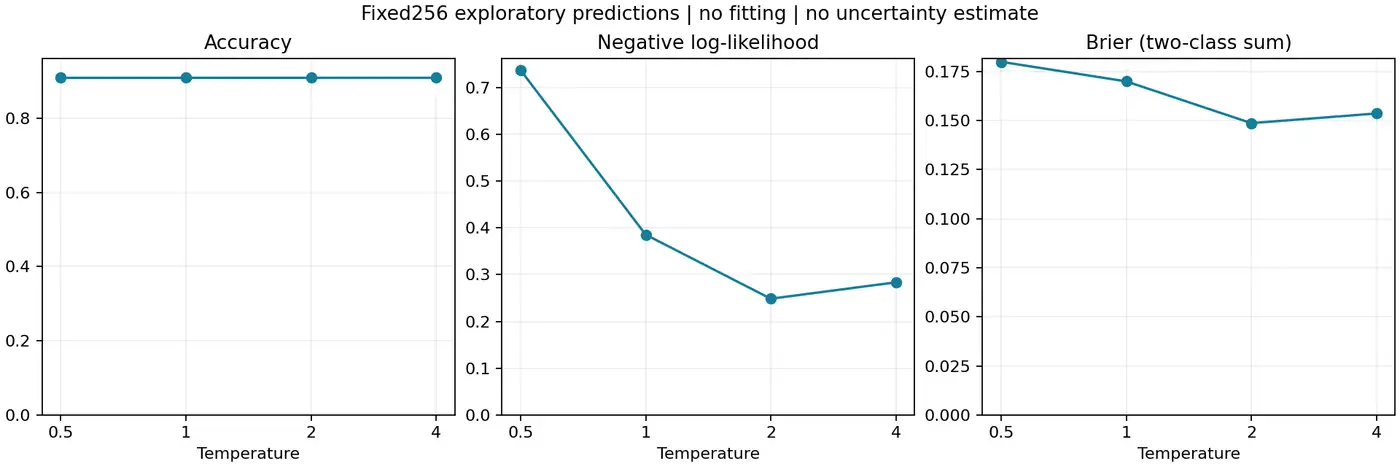
The four accuracys are all 91.02 percent, and the sample predictions are the same, not just the correct totals happen to be the same. From temperature one to two, the loss of both probability decreases; continues to rise to four, and then rises again. This negative result is worth keeping: flattening the distribution does not guarantee continuous improvement of the probability quality. The second in the table is only the lower value observed in the four predetermined conditions, not the recommended parameters obtained by independent calibration.
In order to understand the reason, we divide the NLL into two parts of the correct sample and the wrong sample, and both divide by the complete two hundred and fifty-six. When the temperature is at a time, the contribution of the two parts is about 0.0161 and 0.3692; when the temperature is 2, it becomes 0.0513 and 0.1971. The drop in false contributions exceeds the rise in correct contributions, so the total value is reduced. When the temperature is 4, the correct contribution rises to 0.1627, the wrong contribution drops to 0.1207, and the addition of the two is higher than the temperature two.
This decomposition is an arithmetic interpretation of the same result, not a newly discovered sample causal mechanism. We have not read the wrong text to give semantic tags such as "sarcasm" and "ambiguous", nor do we claim that the error comes from a certain language phenomenon. If this explanation is needed in the future, we should first establish labeling specifications and actual audits, instead of inverting linguistic reasons from the size of the loss.
Independent recalculation and failure investigation
The main program calculates softmax from two scaled fractions. Check the script to calculate the sigmoid from the two types of score difference, then rebuild the NLL with a stable SoftPlus, and rebuild the Brier with twice the single-positive square error. All derived rows, correct numbers, mean and group contributions have been actually checked, and the maximum absolute value deviation is about 2/1 trillion. The input file hash, script hash, execution command and exit code are saved, and the automatic recalculation will not be written as a semantic manual review.
If the predicted category changes, first check whether the temperature is positive, whether the different temperatures are used for the different categories, and whether the code is accidentally re-inferenced. If all probability losses are exactly double the difference, the Brier definition is preferred. If the NLL has infinite values, you should check whether the probability is rounded to zero first, or directly exponentially operated at low precision. Don't sneak the probability of cutting out the abnormality in order to eliminate the abnormality; cropping will change the amount being measured and must be recorded as a new configuration.
This time, the directory cannot write a warning, the log is reserved, and the final image is output normally when the font cache is created for the first time. It does not affect the model output or loss. Registering the environmental prompts and scientific failures separately can avoid all reasoning to re-run all the reasoning to repair the drawing, and also let the reader know which stages have actually been implemented.
Code and instructions for reproducing the results
The complete viewable source code of this article has been disclosed: Directory at the pinned commit、README and run instructions、SOURCE_MAP source map. The archive includes model acquisition and inference entry, probability analysis, independent auditing, fixed dependencies and verification records. The fixed version has been anonymously downloaded, and all files are consistent with the local archives one by one.
The minimum analysis command is python analyze.py && python check_analysis.py, it is expected to generate sample-by-sample temperature records, aggregate results and audit reports. Real model playback use python execute.py smoke --cache .cache112; First run, press README to get fixed resources. The current actual implementation scope is 256 real predictions, four temperature analysis and eight new replays, excluding retraining, full benchmark evaluation or independent confirmation.
Research questions and summary
The aim here was to show a deterministic counterexample on fixed predictions, so we report no confidence intervals and draw no error bars. Estimating differences on new examples would require a prespecified paired analysis and independent evaluation data. Selecting a temperature also requires keeping fitting separate from evaluation. Picking the better-performing temperature now and reporting the gain on these same examples would turn a controlled measurement into a method comparison with selection bias.
A follow-up can ask whether these confident errors cluster in prespecified groups based on length and original label. The existing predictions can answer that exploratory question while leaving the confirmation data untouched. What this experiment establishes is more basic: answer correctness and the quality of the assigned probabilities are distinct. Even at fixed accuracy, probability losses can change, with trade-offs. Saving and checking both dimensions separately gives later calibration and abstention experiments a result they can audit.
References
Search date: 2026-10-30. The following are first-hand sources; the conclusion of the paper, the official realization and the results of this experiment are separately stated.
- Guo, Pleiss, Sun, Weinberger. 2017. On Calibration of Modern Neural Networks,ICML/PMLR 70,1321–1330.
- Author temperature scaling implementation, pinned commit, the temperature division and the Validation Set fitting route.
- DistilBERT SST-2 Official Model Card, fixed checkpoint and label information.
- Stanford NLP SST-2 fixed data version, the data licensing mark is unknown, the source code does not distribute the original statement.
author's work
The following are the author's own products. In addition to scientific research writing, I have also independently developed some daily tools, welcome to understand according to your needs: Daily Expense Journal Used to record revenue and expenditure, arrange budgets and save goals, View on the App Store; One Small Action Help you choose small actions according to time and energy, and record your feelings after completion, View on the App Store. See more technical articles and personal works Details of the work. These works are independent of the experimental conclusions of this paper, and welcome to share the actual use experience.