
Reproduction value: check the ruler first, then discuss the model
The previous baseline put an intuition to the test. DistilBERT correctly classified 233 of 256 fixed sentiment examples, yet its mean confidence was about 98.17%. Now we keep every prediction fixed and change only how we summarize the results. How different is the calibration error when we group the same probabilities into five bins or twenty? If changing the scale gives a more flattering number, what should readers be told?
Here, calibration means that among predictions with similar confidence, the fraction correct matches their mean confidence. For a single prediction made with 90% confidence, all we observe is whether it was right or wrong. Relating that probability to an observed frequency requires a group of predictions and assumptions about sampling. This analysis adds a binning sensitivity table, the full set of paired resampling indices, per-bin statistics, and a record of an independent recalculation. It requires no further training.
What the paper reports In 2017, Guo et al. discussed the calibration and temperature scaling of modern neural networks, and used binning statistics to measure and predict the deviation between Confidence and Accuracy. What we tested: Compare the four types of equal-width bins on only 256 exploration predictions with fixed public checkpoints. Author’s interpretation: Explain the observed cancellation and sparse phenomenon, which can help design the subsequent probability quality experiments; these results do not represent all models, and there is no complete experimental matrix for reproducing the paper.
Core idea: where the absolute value is placed is very important
Expected Calibration Error is usually referred to as ECE. Confidence is drawn from zero to one into several equal-width intervals, and the average probability and accuracy are compared in each interval, and then weighted according to the number of samples. It is a finite sample statistic, and its value depends on the partitioning method.
Here, is the number of boxes, is the total number of samples, is the -th bin’s sample count, is the average maximum category probability in the box, is the mean value of the correct indication value in the box. Enter the shape of logits as , the maximum value of the category dimension after the softmax is obtained, and the Confidence vector of length 256 is obtained. There is no estimable accuracy in the empty box, which is saved as a null value, and the weighted and contributed zero cannot be displayed as "accuracy is zero".
This is different from finding the signed mean difference of all samples first and then taking the absolute value. If there are samples of overconfidence and lack of self-confidence in the same box at the same time, they may cancel each other; after splitting into two boxes, they will take the absolute value respectively, and the offset may be reduced. For tightly nested partitions, the triangle inequality gives:
where, is the original box, Iterate through the sub-boxes that are completely divided, is Confidence, correctness of zero or one. The five boxes are subdivided into ten boxes, and ten boxes are subdivided into twenty boxes to meet this structure, so ECE will not drop under precise arithmetic. However, the fifteen boxes and ten boxes do not constitute this subdivision relationship, and the numerical size cannot be inferred just by the number of boxes. Floating-point errors can also create very small negative differences that must be distinguished from real statistical differences.
A guide to the official implementation
Starting from the definition and formula of the paper, let's look at the author's repository _ECELoss: It first calculates softmax from logits, and then takes the maximum class probability and argmax; then constructs the equidistant boundary, multiplying the absolute mean difference between the absolute mean value of each box. The default parameter for pinned commit is fifteen boxes, and the interval is left open and right closed. The left-closed right-opening convention of the baseline is locally used, and the last box contains the right end point; none of the four types of bins are just on the inner boundary, so the endpoint convention here does not explain the observation difference.
The source map clearly distinguishes: the forwards of the neural network come from a pinned version of Transformers; the basic reasoning and input verification module follows the public source code of the previous article; If the author's GPU temperature fitting process is not changed to a file name, it is called this experiment, and the temperature fit is not performed. The reading order is recommended for protocol, configuration, measurement functions, independent checks, drawing scripts, and finally look at the model forward and original logs.
Minimum experiment: only change one variable
The model is fixed as a DistilBERT SST-2 checkpoint, and the model revision is 714eb0fa89d2f80546fda750413ed43d93601a13, the data revision is 8d51e7e4887a4caaa95b3fbebbf53c0490b58bbb. The Validation Set is sorted by the given identity hashing, and the first 256 are the exploration pool; the other 256 calibration pools and 360 protocol audit pools are not reasoned in this article. The SST-2 has been used in the history series, and the checkpoint author has also reported the validation set result, which cannot be packaged as untested.
The number of four candidate boxes is 5, 10, 15, and 20, and the configuration and protocol are written before running the analysis. Ten boxes are used to connect the baseline, and 15 boxes are convenient for understanding the default caliber implemented by the author; all four items are reported, and the number of "most credible" boxes is not selected according to the results. Freeze label mapping, sample sequence, model probability, truncation, precision and device conditions. No new labels, no artificial semantic classification, and no access to IMDb.
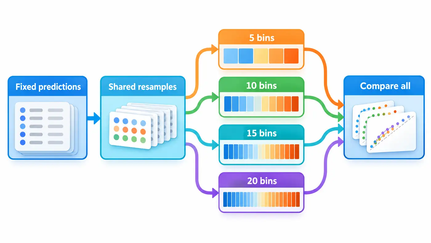
Formal analysis and reuse the sample-by-sample logits and probability of the previous real reasoning, and the file identity is locked through SHA-256. In addition, the CPU reasoning and replay of eight original exploration samples was actually executed, and it is used to check that the source code can still run. It does not add eight test data, nor does it add a formal comparison denominator. The inference is Float32, four threads, and the output shape is eight rows and two columns; the forward takes about 0.070 seconds, the process after importing is about 0.605 seconds, and the process peak is resident in memory about 800MB. The original log of the full 256 official reasoning is reserved with the source code, and the old log date cannot be arbitrarily called today's new run.
Evaluation protocol and results
Pairing self-service resampling means: 256 times are drawn back from the 256 sample indexes at a time, and the four bins use this index together. Seed 113, repeat 2000 times, and save each index and four ECEs. The interval uses 2.5% and 97.5% quantiles of linear interpolation after sorting. In this way, the binning difference under the same sampling disturbance is avoided, and additional noise is avoided when the four methods are each selected.
| equal-width boxes | ECE | Resampling 95% interval | Number of non-empty boxes | Number of samples in the right box |
|---|---|---|---|---|
| 5 | 0.082843 | [0.050882, 0.117772] | 3 | 248 |
| 10 | 0.083705 | [0.053621, 0.119951] | 5 | 242 |
| 15 | 0.083705 | [0.055056, 0.120464] | 6 | 238 |
| 20 | 0.083705 | [0.055361, 0.120251] | 8 | 233 |
Subtracting the five-bin estimate from the twenty-bin estimate gives 0.000862, or about 0.0862 percentage points. The paired interval is approximately [0, 0.012778], with an unrounded lower endpoint just below zero at floating-point precision. This gives little basis for claiming a large change in calibration, and the four overlapping individual intervals do not constitute a formal test of differences. The point estimates for ten, fifteen, and twenty bins agree even though their contents differ. With five bins, the seven predictions with confidence between 0.6 and 0.8 have a mean signed gap of about −0.138. With ten bins, the three in the lower range have a gap of about −0.359, and the four in the upper range have a gap of about +0.028. Separating the two signs reduces cancellation and explains the small increase. Further subdivision did not change the amount of cancellation.
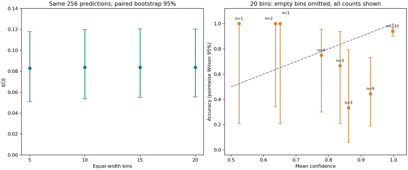
The picture on the left is from the saved resampling results; the picture on the right shows all non-empty boxes under 20 boxes, labeling the denominator, and drawing the box-by-box Wilson interval of Accuracy. All figures in the figure are generated by the log, and the icon of the method diagram does not bear the quantitative evidence. The non-empty box denominator of the 20 boxes is 1, 2, 1, 4, 3, 3, 9, 233, a total of 256.
Failure investigation: the small box is not a more detailed truth
The most important investigation sequence is not the style of the graph first, but to confirm the probability object, denominator and boundary. The first verification probability is obtained by the same group of logits, and the predicted category is consistent with the correctness map; then the sum of the number of samples in each box is still 256, and each sample is exactly in one box. The maximum probability of two classifications is at least one-half, and a large number of empty boxes in the first half are structural phenomena, not data loss. After directly deleting the empty box, the remaining boxes are equally averaged, and the indicators will be quietly replaced.
Then look at each box of evidence. A box with only one sample, its observation accuracy can only be zero or one; it is easy to exaggerate the explanation when it is drawn as an exact point without the denominator. The Wilson interval is only for the accuracy in the box, not the interval of the average Confidence, and it is not the simultaneous confidence band of the entire calibration function. This paper uses independent row resampling; if there is a correlation or near repetition between the text, the interval may be underestimated and uncertainty, so it is only used as a sensitivity statement under the distribution of empirical data, and does not claim coverage guarantee.
The independent script does not import the measurement function, but reconstructs the probability and prediction from the two-dimensional Logits, uses the interval comparison and re-binding, uses the sum of the signed residuals to calculate the ECE, and then checks the 8000 resampled values and interval endpoints one by one. The input hash, script, command, and exit code are reserved. This is automatic arithmetic verification, not artificial gold label or semantic review. The analysis took about 4.45 seconds, and the peak resident memory was about 63.7MB; the statistical and model inference resources were recorded separately, and the plot resources were not measured separately.
Code and instructions for reproducing the results
public and anonymous verification Source tree at the pinned revision、README and SOURCE_MAP. This article provides complete inference entry, fixed resource acquisition and verification module, statistical scripts, drawing scripts, dependency records and source code maps. The minimum command is as follows, can be executed in the source code directory, no need to re-download the model:
python analyze.py && python check_analysis.py
It is expected to obtain the results of four bins, all resampling indexes and independent audit records. When you need to verify the real model path, press README to obtain fixed resources and run eight Smokes; the download cache must be checked through the resource lock. The package does not distribute the original emotional text or model weights, nor does it depend on the absolute path on the author's computer. The code and statistical records can be browsed publicly, and the compressed package is only responsible for the local archive, and is not used as the unique source code of the blog.
It is also necessary to prevent re-sampling for re-collecting data. The repetition of the sampling index is part of the algorithm design: the same line is drawn three times in a certain repetition, and the weight is contributed three times; the line that is not drawn is temporarily not contributed. It does not create new independent texts, let alone make up the language style that the original data does not cover. The advantage of saving all indexes is that others can not believe the version commitment of the random number generator, and directly use the same index to review each statistics.
Another negative result worthy of preservation is that after the binning is thinner, the overall indicator is almost unmoved, but the Accuracy in the right box has changed from about 90% to about 94%. It is not that the same group of samples has become more reliable, but the interval has been reduced from a wider range to a higher Confidence range, and the members have been replaced. Therefore, when comparing the accuracy of a "last box" across bins, the interpretation of the same group cannot be applied; it is necessary to display the boundary, identity and quantity at the same time. All box-by-box members can recover from open probability and clear boundaries without sharing the original sentence.
For engineering readers, the most practical delivery convention is to let the indicator name carry the agreement: the description is the maximum category probability calibration, the isometric bin, sample weighting, and endpoint attribution. For graduate students, it is more important to describe the estimation object: the binning deviation of the model on this empirical sample is estimated here, not the exact integration of the potential overall calibration function. Whether to maintain the same conclusion after expanding the data, still needs new experimental tests.
Research questions and summary
This controlled control did not find a clear boundary that can greatly change the ECE of this group, but found a high concentration of high-confidence samples and a clear boundary for low denominator intervals. The question that can be verified in the future is: when the predicted category remains the same and only changes the probability distribution, do the Negative Log-likelihood and the Brier score give the same order? This problem requires pre-specified transformations and a complete report of candidates, rather than changing the probability first and then picking the metrics that support the most conclusions.
The conclusions that can be left in this article are limited and clear: the ECE dependence statistical protocol of the same group of forecasts. The research record should also keep the probability, denominator, interval convention, sampling method and failure boundary at the same time, so that the reader can change the measurement protocol independently, instead of accepting only one conclusion that reserves three decimals.
References
Search and code verification date: 2026-10-29.
- Guo, Pleiss, Sun, Weinberger. 2017. On Calibration of Modern Neural Networks,ICML/PMLR. In this paper, according to the definition of the boxed index, we do not claim to reproduce all the experiments.
- Geoff Pleiss, author of the paper Temperature_scaling Fixed commit source code, MIT license; the default number of boxes corresponds to this implementation.
- Hugging Face, DistilBERT SST-2 Fixed Model Card, checkpoint identity, tags and task range.
- Stanford NLP, SST-2 Data Fixed Version, data division and acquisition entry; the original text is not distributed with this article.
Apps by the author
The following is the author's own product promotion. In addition to writing scientific research blogs, I also independently develop daily gadgets, welcome to understand according to your own needs: Daily Expense Journal Used to record revenue and expenditure, arrange budget and saving goals, View on the App Store; One Small Action Help choose small actions based on time and energy, and record how you feel after completion, View on the App Store. More technical articles and personal works are available Author website. These works are independent of the experimental conclusions of this article and do not represent the recommendation of the author of the paper or the research institution.