- Date: 2026-09-09
- For graduate students, early-career researchers and research engineers
Abstract
If we compress weights from 32 bits to 4, does inference run eight times faster? We measure three effects separately on the same model and test sequence: storage savings, degradation in predicted probabilities, and computational overhead. After examining LLM.int8(), GPTQ, AWQ, and their official source code, we packed real integers and ran floating-point inference in a reproducible synthetic token model. The file shrank, but dequantizing on each pass slowed the forward computation. These local measurements test the mechanism without replicating the large-model results in the papers.
Recover value: first clarify "what is quantified"
Quantization after training, that is, PTQ, is to reduce the representation accuracy on the existing weight, and usually do not retrain the entire model. W4A16 represents four-bit weights, sixteen-bit activation, and activation is the intermediate value in the forward pass; it does not promise that all multiplications will be executed in four digits. Storage format, multiplication input, accumulated precision and output precision must be recorded separately.
Paper report: Dettmers et al. LLM.int8() combines the decomposition of vector scale and mixed precision, and hand over the feature dimension where the outlier values are located to the high-precision branch. It studies the effect of outliers on calculations in a specific model, and cannot be simplified to "convert all weights directly to INT8". Original paper
The GPTQ of Frantar et al. uses approximate second-order information to compensate for the remaining weights after quantifying a portion of the weight. The AWQ of Lin et al. is activated and searches the channel scale to protect important weights. Both go beyond direct rounding; this paper implements the rounding baseline that is easy to compare, and these two algorithms have not been implemented. GPTQ full text、AWQ full text
The four digits are not only an integer mesh evenly. NF4 is another four-bit data type, and NF4, INT4 and "four-bit calculations" cannot be used as synonyms. When using the framework, you should save the quantization type and the calculation dtype, not just one load_in_4bit switch. official statement
Core Ideas and Formulas: Rounding errors will be enlarged by input
This time, we use symmetric quantization for each group of weights:
is the bit width, for the group scale, for integer numbers, is the approximate weight after recovery. The all-zero group order scale is one to avoid division of zero. In this example, INT4 uses fifteen levels of negative seven to seven; add eight codes during storage, and two four-digit codes are loaded into one byte, and one unused code is reserved. This is a symmetric baseline that is deliberately selected, not equivalent to all INT4 formats.
If linear layer writing , then shape is [N,d]、 For [o,d], the output is [N,o]. quantization , so equal mean squared weight error need not give equal output error. Construct a diagonal input matrix with amplitudes 100 and 1. In each of two trials, add an error of 0.1 to just the corresponding weight. Both trials have a mean squared weight error of 0.005, yet their squared output errors are 100 and 0.01. The script checks this counterexample.
Group scales also have costs. When the entire tensor shares a scale, a few large amplitudes may increase the interval of the grid, so that the small weight is squeezed near zero; the team leader can partially adapt to the scope, but it needs to save more scales, and may change the kernel alignment and access. During comparison, the bit width, group leader, grouping axis and metadata accuracy should be written at the same time, and the "four bits" in the file name should not only be used as an experimental configuration.
It explains why the calibration requires input distributions: The Calibration Set is the data prepared for the estimation of activation or quantization parameters, and should not be used as the Test Set. In this paper, the scale is determined only by the absolute maximum of the weight, and there is no calibration sample; this makes the protocol simple and limits its ability to deal with sensitive channels.
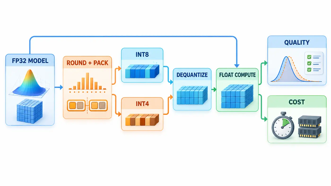
The blue bypass in the figure is a floating point baseline, and the integer branch is inverse quantized first, and then entered the floating point calculation. The cost evaluation includes the byte and forward timing of the packaged file; the terminal arrow indicates the summary measurement, not only the memory is measured after the calculation is over.
Guide to the official implementation: numerical simulation and deployment core are separated
from GPTQ gptq.py Read add_batch, see how the input accumulates into the second-order statistical matrix; read again fasterquant The damping, Cholesky decomposition and column-by-column error compensation. Check the group leader and the activation sequential parameters, as they change the quantization process. algorithm source code
follow-up opt.py The forward hook find the calibration entrance, and then look at opt_eval blocks and label shifts. It is only confusing to understand "Which tokens are scored". The quantitative algorithms, evaluation scripts and the underlying kernel provided by the repository are different levels. Evaluation source code、Official repository
AWQ auto_scale.py Search candidate scales, and use the difference selection scheme before and after quantization; this is an offline search, not a retraining language model. quantizer.py Then it is clear to distinguish between analog quantization and real module replacement, the latter enters WQLinear. Scale Search、quantization source code
Look at last qmodule.py packaged with forward: It dispatches matrix vectors or matrix CUDA paths by input scale. How to arrange low-bit data, where to inverse quantify, and which kernel is called is connected to the actual speed. This article reads the retrieval day main, the commit has not been locked, and these CUDA paths have not been run, and the compatibility is subject to manual verification. Module source code
Minimum experiment: training first, then fixed quantitative control
code/minimal_quantization.py Use NumPy to train a two tokens context model: sixteen vocabulary, each tokens is embedded in eight dimensions, and after splicing, the 64-dimensional hyperbolic tangent hidden layer is output, and the output is 16 types, a total of 2,256 parameters. enter as [B,2], the output is [B,16]; This is not a Transformer, and there is no pre-training of natural language.
The data generation rule is based on the probability of 90%, and the successor is generated according to the parity of the previous tokens and the previous tokens, and the rest of the situation is even and random. There are two hundred and fifty-six, sixty-four, and one hundred and twenty-eight independent sequences for training, development and testing, respectively, each with a length of 34. The first two tokens are only the context, the latter thirty-two scores; the complete sequence is not repeated across the collection, but the short context and the rules are shared, so only the same distribution prediction is tested.
The initialization seeds are fixed at 68, 69, and 70, each training is 800 steps, the batch size is 128, and the Adam learning rate is 0.01. In the scheduled four checkpoints, use the development set Negative Log-likelihood, that is, NLL, select the model; all three seeds are selected 800 steps. Quantization formulas are pre-determined, and the test set is not involved in the selection.
python3 code/minimal_quantization.py > code/smoke_test.txt
python3 code/audit_results.py
python3 -m py_compile code/minimal_quantization.py code/audit_results.py
Environment and installation steps see code/README.md; This time, I actually use Python 3.12.14, NumPy 2.3.5, macOS ARM64 CPU. Embedded and two-layer matrix participate in quantization, bias reserves FP32. G32 refers to flattening in the order of continuous storage, each thirty-two values, which may be across rows; it is not equivalent to the official grouping of input channels.
| Set up | Mean of test confusion ± standard deviation | Model load bytes |
|---|---|---|
| FP32 | 1.9580 ± 0.0141 | 9024 |
| INT8,G32 | 1.9583 ± 0.0141 | 2768 |
| INT4, one set of each tensor | 1.9924 ± 0.0336 | 1420 |
| INT4,G32 | 1.9759 ± 0.0134 | 1680 |
The above is the actual verification. "±" is the standard deviation of the three initialized samples, not Confidence interval . Loads include integer weights, FP32 scales and offsets, and do not include shape lists and file system overhead. The four-bit weight body of G32 occupies 1088 bytes, the scale occupies 272 bytes, and the bias occupies 320 bytes; so the overall compression ratio is about 5.37, not eight times.
The single-sample front median of the seed 68, the floating-point baseline is about 3.50 microseconds; if the four-digit group is unpacked each time and re-quantified, it is about 22.42 microseconds; 3.71 microseconds. Each path is preheated 20 times, and the measurement is 100 times. The original sample and the nine-decade digits have been saved. This is a tiny CPU forward, excluding disk loading, sampling or full generation loops, nor is it an integer core speed.
Syntax checking and CPU Smoke Test pass; independently audit twelve sets of models from disk, recalculate the NLL of 4,096 tokens per group, and check the number of bytes, confusion and development set points. The maximum error of the finite difference of one of the five types of parameters is about , is not an exhaustive proof of all gradients.
Evaluation protocol: quality, delay and video memory have a denominator
Confusion is defined as , is the NLL of the effective target tokens, is the total number of targets. The loss and quantity are accumulated first and then exponential, and the confusion of different length batches cannot be averaged. The formal language model should be fixed tokenizer, document connection rules, context length and sliding window step size; the overlapping part only provides context, and cannot be scored repeatedly. The count should directly check the valid label after shift. Official review description
The speed is to measure the Prompt pre-fill and tokens decoding separately, and fix the batch, input and output length, cache accuracy, device and software version. GPU timing needs to be warmed up and synchronized, and the number of repetitions and distribution are reported. The AWQ supporting system combines real-time inverse quantization and kernel fusion; this paper restores the implementation of the entire weight matrix one after another, and it is impossible to judge the speed of AWQ according to this. AWQ system part
To move from this example to an official experiment, choose a model the repository explicitly supports. Pin the weights, tokenizer, and code version, and run the floating-point evaluation before quantizing. Fix the calibration documents, sample count, and truncation rule, then vary bit width or group size one at a time under the paper’s settings. Integrate the deployment kernel last. Report quantization time, peak resource use during calibration, and inference resource use separately so a claim about loading the model once does not hide the cost of offline preparation.
The video memory budget should include quantized weights, scales and zeros, unquantified layers, key-value caches and temporary workspaces. The key-value cache holds the attention state of the processed tokens, and does not automatically shrink because of the quantization weight. In this example, there is no attention cache, and the restored parameter array still accounts for 9024 bytes; the process also keeps the baseline and the intermediate array at the same time, so this number is not peak memory. The machine does not perform GPU inference, and the peak video memory and natural language confusion are both manually verified.
Failure investigation: priority to find agreement differences
If the confusion suddenly skyrockets, first verify the package round-trip, scale order, zero point and matrix direction, and then see if the unsupported module is incorrectly quantified. Compare the floating-point and restored output layer by layer, and you can distinguish the encoding error from the normal rounding error; it is not enough to check the file to load.
If the model becomes smaller but slows down, confirm whether the floating-point dungeon is constructed at each step, back to the general operator, or the test scale is too small and the overhead is dominated by the invocation. This time, the dequantization cost has indeed been observed, but the microsecond-level results are also affected by the system scheduling; the fastest single-shot value cannot be regarded as a stable throughput.
Grouping is also not guaranteed to be better every time. In the seed 70, the entire tensor INT4 has a puzzle of 1.9561 and G32 is 1.9612, which is different from the order of the three seed mean. The weight error and probability loss do not correspond one-to-one, and the loss should be kept one by one, and pairing and comparison should be made on the same sequence.
Tokens in short sequences are not independent. If you want to add an error line to the loss difference before and after quantization, you should first aggregate according to the entire sequence, and then do pair resampling on the sequence; treating more than 4,000 tokens as independent samples will exaggerate the accuracy of evidence. The current three seed shared data segmentation, the standard deviation only describes the training initialization and sampling changes, and does not represent the uncertainty after the corpus is changed. The original sequence and tokens losses have been saved and can support subsequent audits.
Questions for further research
The authors infer that the group benefit may depend on the dynamic range within the group, and may also be offset by the sensitivity of different layers. The next step is to keep the total byte budget the same, compare shorten the length of the group, improve the width of the sensitive layer, and retain a small amount of high-precision layers; otherwise the quality improvement brought by the additional scale is not free.
Then move the calibration data from the same field to the different realms, keep the test documents isolated, and compare the output errors of GPTQ and AWQ and the task Accuracy . If the confusion is close and the structured response degradation, it means that the average tokens loss has omitted important failure slices; this requires real task evidence, and the current toy model cannot answer.
Summary
This time, the replayable link from weight rounding, integer packaging to independent probability evaluation has been completed, and it is verified that the volume reduction and speed increase need to be proved separately. The paper gives a method to reduce the quantization error. The source code displays the calculation path, while the trusted experiment needs to save the bit width, scale, scoring protocol and real execution boundary at the same time.
References
Search date: 2026-09-09. The links of the text are all first-hand sources of actual opening; the dynamic code is not locked for submission, and the complete paper is reproduced for manual verification.
- Tim Dettmers、Mike Lewis、Younes Belkada、Luke Zettlemoyer,2022, LLM.int8(): 8-bit Matrix Multiplication for Transformers at Scale,arXiv v2,NeurIPS 2022.
- Elias Frantar、Saleh Ashkboos、Torsten Hoefler、Dan Alistarh,2023, GPTQ: Accurate Post-Training Quantization for Generative Pre-trained Transformers, arXiv V2, ICLR 2023; preprints were first published in 2022.
- Ji Lin, Jiaming Tang et al., 2024, AWQ: Activation-aware Weight Quantization for LLM Compression and Acceleration, MLSys 2024; pre-printed edition was first published in 2023, this time reading V6 (2026 revision), the title of the HTML body also includes On-Device.
- author team, GPTQ official repository、AWQ official repository, read the search day main, see the text for the specific module.
- Hugging Face, Bitsandbytes Quantitative Documentation、Evaluation of the Confusedness of Fixed Length Model, dynamic documents.