
Research question: what changes when input length is the only intervention?
In the previous experiment, we applied a classifier trained on short sentences to full-length film reviews. Accuracy and probability quality told different stories. There was also a limit on what the classifier could see: 512 tokens. A token is a unit produced by the tokenizer and may cover only part of an English word. A review can easily exceed 512 tokens. The classifier still returns two probabilities, even if it never saw the end.
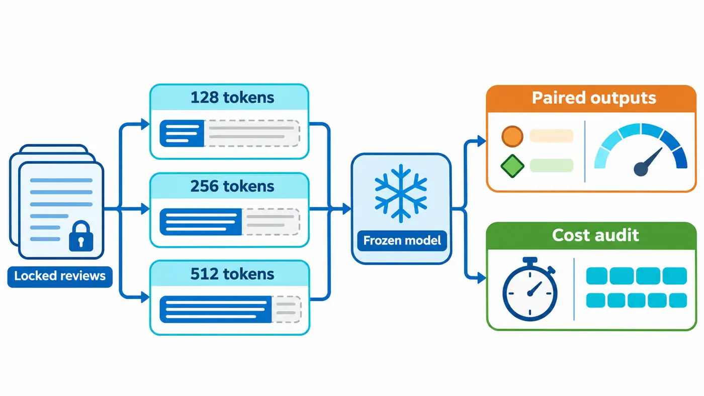
Take the same review and shorten the input. Does the classifier become more or less certain, or does it actually change its answer? We held the model, tokenizer, sample IDs, labels, batch order and numerical precision fixed. Only the maximum input length varied: 128, 256 or 512 tokens. The experiment produced 3,000 paired predictions, a truncation count for each input and an independent audit script.
Shortening the input changed both confidence and the predicted label. Relative to the 512-token run, labels flipped on 139 reviews at 128 tokens and 47 at 256. These counts describe one fixed model and one exploratory sample. We did not relabel the shortened reviews or check whether the omitted passages contained a reversal or a conclusion.
Where truncation changes the prediction
Temperature scaling acts on scores the model has already produced. Truncation happens before the forward pass. Removing the last tokens can change what the attention layers see, the pooled representation and the resulting class scores. Two runs can predict the same label with different probabilities. They can also be equally confident in opposite labels. The tokenizer documentation distinguishes padding, which aligns lengths within a batch, from truncation, which limits the input the model actually reads. Transformers Documentation
Let the original sequence of tokens, excluding special tokens, be , with length . We truncate on the right and reserve two positions for the start and end tokens:
Among represent samples, is the length limit including special tokens, and is the number of tokens withheld from the model. This measures how much text was removed. It says nothing about the meaning of that text. To verify that truncation really occurred on the right, the program compares each input with the corresponding prefix of the full token sequence.
The model returns , with one column for negative sentiment and one for positive. We use probabilities without temperature adjustment:
here denotes the class. Confidence is the larger of the two probabilities. Ties go to the lower label index. Negative log-likelihood uses the probability assigned to the label of the original, full review. It measures the loss on the original task given only the visible prefix. Whether the prefix deserves that same label is a separate question.
We compare each shorter run with the longest run using the label-flip rate and the mean absolute change in confidence:
denotes the 1,000 exploratory examples. Taking the absolute value keeps increases and decreases from cancelling each other out. The mean can still hide a few large shifts, so it tells us little about any one review.
A guide to the official implementation
Start with the pinned model card. It describes a DistilBERT classifier fine-tuned on English sentiment data. Then follow the classification forward pass at the pinned commit to see how the head turns hidden states into two scores. Finally, inspect the fast tokenizer’s truncation settings and batch encoding. The source map records the commits, file locations, licenses and local calls we verified. Model card
We use the official classifier directly. The teaching code fixes the sample IDs, iterates over input lengths, saves predictions and computes metrics. That separation lets you check the network, inputs and statistics independently. We also compared the framework files byte for byte with the installed files, since matching version numbers alone cannot rule out local changes.
A minimal experiment and evaluation protocol
We reused the three IMDb pools from the previous article. Their IDs were frozen before the first prediction. Reviews were grouped by film and deduplicated using a normalized-text digest, then allocated in stable hash order to pools of 1,000. Only the exploration pool supplied text and labels for this run. We did not fit on the target-domain calibration pool. The final confirmation pool stays sealed until the end of the series. Deduplication by film changed the sampling distribution, so results on these 1,000 reviews should not be reported as a score on the full official test set.
Earlier studies used the source-domain SST-2 data. Resplitting it cannot erase that history. The checkpoint and tokenizer share a pinned revision, and we verified the digest of the original official IMDb archive. Public reviews may have appeared in pretraining, so we cannot establish zero contamination. The archive stays in a shared cache. The release distributes identity digests and derived predictions, with the full review texts available from their original source.
Before running the experiment, we fixed the protocol: report all three lengths, process them from shortest to longest, use batches of 16 and four CPU threads, and run in single precision with evaluation mode, deterministic algorithms and the standard attention implementation. Each condition started with an eight-example smoke test to estimate the cost of processing all 1,000 reviews. We did no training, target-domain calibration or prompt search. We also reran inference at 512 tokens to obtain a fresh comparison.
Which reviews changed labels?
| Token limit | Correct against original label | Label flips vs. 512 tokens | Mean absolute change in confidence | Negative Log-Likelihood |
|---|---|---|---|---|
| 128 | 829/1000 | 139 | 0.03141 | 0.74291 |
| 256 | 877/1000 | 47 | 0.01667 | 0.51091 |
| 512 | 890/1000 | 0 | 0 | 0.44102 |
The table reports measurements from this run. Mean confidence shifted by about three percentage points, yet nearly 14% of predictions flipped. Confidence retains only the larger probability. It discards the identity of the class that received it, so two confident predictions in opposite directions can look almost identical on this metric. To monitor confidence drift, save the full probability vector and the predicted class alongside it.
Going from the longest to the shortest input turned 100 correct answers into errors and 39 errors into correct answers, a net loss of 61 correct predictions. At the middle budget the corresponding counts were 30 and 17. With two classes and a fixed label, exactly one of two disagreeing predictions must be correct. The audit script uses this identity to check the flip count. It is an arithmetic check on predictions, not a human review of the text.
At the prespecified raw-confidence threshold of 0.9, the three runs accepted 937, 937 and 945 reviews, respectively. Among those accepted, 142, 97 and 89 predictions were wrong. The acceptance counts look much alike, yet the errors differ considerably. We kept the threshold fixed throughout. This exploratory check gives no population-level risk guarantee.
What is discarded and what is saved
At the three budgets, 895, 425 and 109 reviews were truncated. The corresponding numbers of discarded tokens were 168,090, 84,526 and 25,305. Even at 512 tokens, the model missed part of some reviews. The longest run is therefore a reference budget. Comparing against it cannot measure the total loss from truncation relative to reading every review in full.
The inference loops took about 9.88, 22.89 and 56.18 seconds. These times include batch encoding and model computation. Full-text tokenization for the length audit, model loading and data reads took place separately. The logs also record total wall time, peak process memory, batch shapes and padding-token counts. Peak memory accumulated within one process, so it cannot serve as an independent memory measurement for each length.
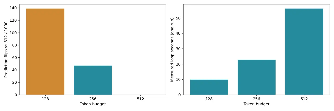
We measured the three conditions once, in a fixed order, without randomized ordering, repeat runs or confidence intervals. The timings do not support a precise hardware speedup claim. With dynamic padding, the longest review in each batch also affects cost. The total count of retained tokens therefore differs from the padded workload. When comparing timings, match the batches and thread counts as well as the length limit.
Troubleshooting and limits of the evidence
The full-length token-counting pass warned that some sequences exceeded the model limit. No overlong sequence entered the model: the forward inputs were truncated again for each budget, tensor shapes were logged, and per-example assertions checked the prefix after excluding special tokens. If you see this warning during an actual forward pass, inspect input lengths and positional-encoding limits before suppressing it.
Keeping a label fixed does not establish that a prefix expresses the same sentiment as the full review. Here the official label measures how well a reader of the prefix can predict the original task label. We did not obtain independent labels for prefixes, inspect removed negations or attribute flips to a twist at the ending. Testing that explanation would require annotation guidelines, a set of passages for review and actual human judgments.
The independent audit starts from the two score columns without importing the main evaluation function. It reconstructs normalized probabilities, correct counts, losses, flips and truncation counts, and verifies the exploration-pool IDs. All 3,000 records passed. This supports the internal consistency of the files. Source provenance and the model’s understanding of the text require other evidence. Here, time and memory are measured quantities, while possible semantic explanations remain hypotheses.
Code and instructions for reproducing the results
Open The source code of this fixed version, press README reproduction instructions run; SOURCE_MAP source map List the corresponding relationship with the local module.
The minimum offline command is python run.py analyze && python audit.py. This reconstructs the results and independently checks the saved scores. For fresh inference, install the pinned dependencies, verify the downloads, then run the smoke test and full experiment at each length. The outputs include per-example scores, input digests, grouped results and environment records. For this article we actually ran eight pilot examples and 1,000 full inferences at each length.
Can be checked and summarized
Two questions follow. Are flips concentrated among reviews that were actually truncated? Do large confidence shifts with an unchanged label disrupt an existing abstention rule? Fix the groups, change threshold and primary statistic before examining the designated development data. To compare windows from the start and end of a review, hold the token budget and number of windows constant so that extra computation cannot masquerade as better window selection.
On these 1,000 fixed reviews, shorter inputs changed both labels and probabilities. Inference sped up and fewer answers matched the original labels overall, although some reviews became correct with less text. More context did not win on every example, and high confidence alone could not establish that truncation was harmless. Saving each input’s identity, length and prediction makes those exceptions possible to investigate.
References
Sources checked on 2026-11-18. The text distinguishes published findings, official API behavior and measurements from this run.
- Andrew L. Maas、Raymond E. Daly、Peter T. Pham、Dan Huang、Andrew Y. Ng、Christopher Potts,2011, Learning Word Vectors for Sentiment Analysis, ACL, IMDb data source.
- Hugging Face, DistilBERT SST-2 Model Card, the actual weight version and the file summary can be found in the source code locking record.
- Hugging Face,Transformers 4.49.0, Padding and truncation, enter the control rules.
- Hugging Face, Fixed Submitted Classifier Implementation, the specific calls and permissions are shown in the source map.
- Chuan Guo、Geoff Pleiss、Yu Sun、Kilian Q. Weinberger,2017, On Calibration of Modern Neural Networks, ICML, Probabilistic Calibration Background; this article does not re-fit the temperature.
Apps by the author
I also build small tools for everyday life. Here are two of my apps:
- Daily Expense Journal: Track your income and spending, plan a budget and set savings goals. View on the App Store.
- One Small Action: Pick a small action that fits the time and energy you have today, then record how it felt and what you noticed. View on the App Store.
Find more articles and projects on my website: zffjzz.top. I’d love to hear how the apps work for you and what I could improve.