The confidence lab: from model confidence to testing when to abstain

Ten less mistakes, how stable can this number stand?
There are three hundred and sixty-tagged movie review short sentences, and the model is allowed to answer 200 of them. Give the model with the most certainty to queue up first, and answer eight wrong sentences incorrectly; queue up according to the list that was disrupted in advance, and answer eighteen incorrectly. The difference between the two lists is easy to calculate, but the difficulty is to explain this ten. If the sentence that was drawn into the audit pool is slightly different, a problem may occur twice, or it may be completely absent. We wonder if the sample change of this degree is enough to make the difference disappear?
The previous article compares three confidence scores on the same two-class header, and the three sorts are not even exchanged for the position of a pair of sentences. Continuing to change the score name does not add evidence. This time, only the number of occurrences of each sentence in the evaluation batch is changed. Models, original labels, sample budgets, two queuing rules, and main comparison locations are all fixed. The new product is a one-by-one-receiving risk difference and interval record, and readers can chase from a seemingly stable point to an extreme situation where only one sentence is accepted.
The answers obtained in this actual verification depend on the denominator. When accepting 270 sentences, the range of confidence orders with few errors is about 3.7 samples per 100 answered samples, and the matching interval is still above zero. When only eighteen sentences are accepted, the point estimate is larger, but the lower edge of the interval has already encountered zeros. Each of the coverage points is reserved below, and the main conclusion is read-only for pre-specified locations.
Research objects and papers
The selective classification gives an additional decision to a well-trained classifier, i.e. whether to deliver the answer this time. Coverage calculates how many answers are delivered, and selective risk measures the conditional error rate in the delivered answers. Geifman and El-Yaniv distinguished these two quantities in the original paper of 2017, and also studied how to use independent data to control risks. They reported image classification experiments. Borrowing this pair of definitions, the strategy of comparing two fixed budgets in the English emotional classification is estimating only the sample fluctuation, and the risk control procedure of the paper is not executed.
The data comes from the SST-2 verification division disclosed by the Stanford team. At the beginning of the project, three pools of exploration, calibration and protocol audit have been drawn in the hash order of the sample identity. This time, I will only reason about the last three hundred and sixty sentences. SST-2 has been used in the preface study, and the number of errors in the overall correctness of the audit pool and even the main location has long been recorded. Before the resampling protocol is written before the calculation interval, today's analysis options can be constrained; these old sentences are still evidence of historical development. The IMDb confirmation pool is not read throughout the whole process, and no one changes the label according to the text meaning.
From one sentence to a pair of risks
give Write down whether the prediction of the model is different from the official label, and the difference is recorded as , the same is denoted as zero. The two class scores of the model are normalized by softmax, and the larger probability is used to arrange the letter order. The other queue is arranged in ascending order of the hash value of fixed prefix and sample number, in the order of the previous experiment. Hash operation read-only identity, neither sees emotional tags nor predicts. Comparing this can be reconstructed to the baseline that can be reconstructed sentence by sentence. If all possible random lists are averaged, the reference object will change accordingly.
here is the -th sample ID in a given queue, is the number of acceptance, and Represents fixed scrambling and confidence sorting, respectively. Income There are fewer errors left for confidence ordering under the same answer budget. Both groups of denominators are the actual number of sentences accepted. When the coverage rate is calculated, the total number of 360 is used as the denominator. Both error counts are zero, and the risk and difference are written to null values when the number of acceptances is zero; refuses all answers to provide any observations about the quality of the delivered answers.
Take the main position and calculate it again. The coverage of the two arms is both 75%, the risk of disrupting the queue is about 6.67%, and the confidence queue is about 2.96%. Subtract directly to get 3.70 percentage points. Divide ten by three hundred and sixty, and it becomes the ratio of the whole batch to arrive in the sample with fewer missed answers. Both denominators can serve research, and only the former one corresponds to the longitudinal axis of this article. It is also not possible to interpret "ten mistakes" as two lists, and only ten samples are exchanged, and the correct samples that are exchanged in and out do not appear in the difference.
Minimum Experiment and Pairing Protocol
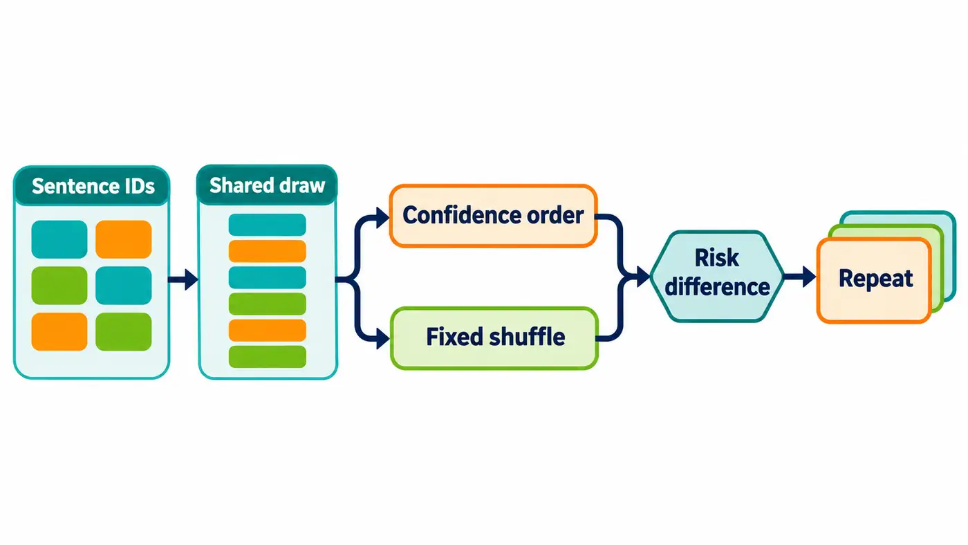
Write three hundred and sixty identities on the card. Draw one, write down the number, put it back, and draw again, until it is full 360 times. Make a copy of this record, and get a queue on the left and right. A sentence is drawn three times, with three identical predictions and labels on both sides. Sentences lined up near the cutoff position may be squeezed out by it, so each time the prefix is re-cut on the new sample. Only drawing lots from the 270 sentences originally accepted will exclude the entry and exit of the edge of the list from the estimate.
If it is changed to one left and right, the same error is absent on one side and the other side is repeated, and the difference between the two batches of fluctuations in difficulty is mixed. Similarly, each strategy is calculated for one interval, and then the upper bound is subtracted from the other lower bound, and the difference distribution on the same batch of questions cannot be restored. The pairing requirement is shared by the sampling index, allowing the two strategies to finally accept different sentences. Only by retaining this can we have the opportunity to observe the benefits caused by the sorting itself.
Fixed random seeds were one hundred and twenty-four, repeated 4,000 times. Each round is counted once for all non-empty acceptance numbers, and the 4,000% difference between the same acceptance number is taken 2.5% and 97.5th in terms of 97.5%. This is the approximate 95% Confidence interval of the percentile self-help method. It uses sentences as an independent sampling unit, and simulates resampling with the experience distribution of the existing pool. The 360 identities of the original audit pool have different text summaries; if multiple fragments are from the same review, their errors may be related; this experiment is not clustered according to the original film review, and the sensitivity of the interval to this dependence is still unknown.
Fixed seeds control which cards the reader draws when recalculating. Increasing the number of repetitions can reduce the simulation error of the quantile, and the original test information is still only 360 sentences. Each line in the four thousand rounds carries the features learned from the same model and the same set of official tags. The model differences introduced by retraining, vocabulary changes after domain change, and disputes caused by label definitions have not entered this interval. The estimated object is the risk difference of two fixed sorts on such samples.
The actual result
| Acceptance / 360 | Errors after ranking by confidence | Errors in the fixed shuffled order | Gain (percentage points) | 95% point-by-point interval (percent points) |
|---|---|---|---|---|
| 1 | 0 | 0 | 0.00 | [0.00, 0.00] |
| 18 | 0 | 1 | 5.56 | [0.00, 22.22] |
| 36 | 0 | 2 | 5.56 | [0.00, 13.89] |
| 90 | 0 | 5 | 5.56 | [1.11, 10.00] |
| 180 | 3 | 12 | 5.00 | [1.11, 8.89] |
| 270 | 8 | 18 | 3.70 | [1.11, 6.30] |
| 324 | 17 | 27 | 3.09 | [0.93, 4.94] |
| 360 | 30 | 30 | 0.00 | [0.00, 0.00] |
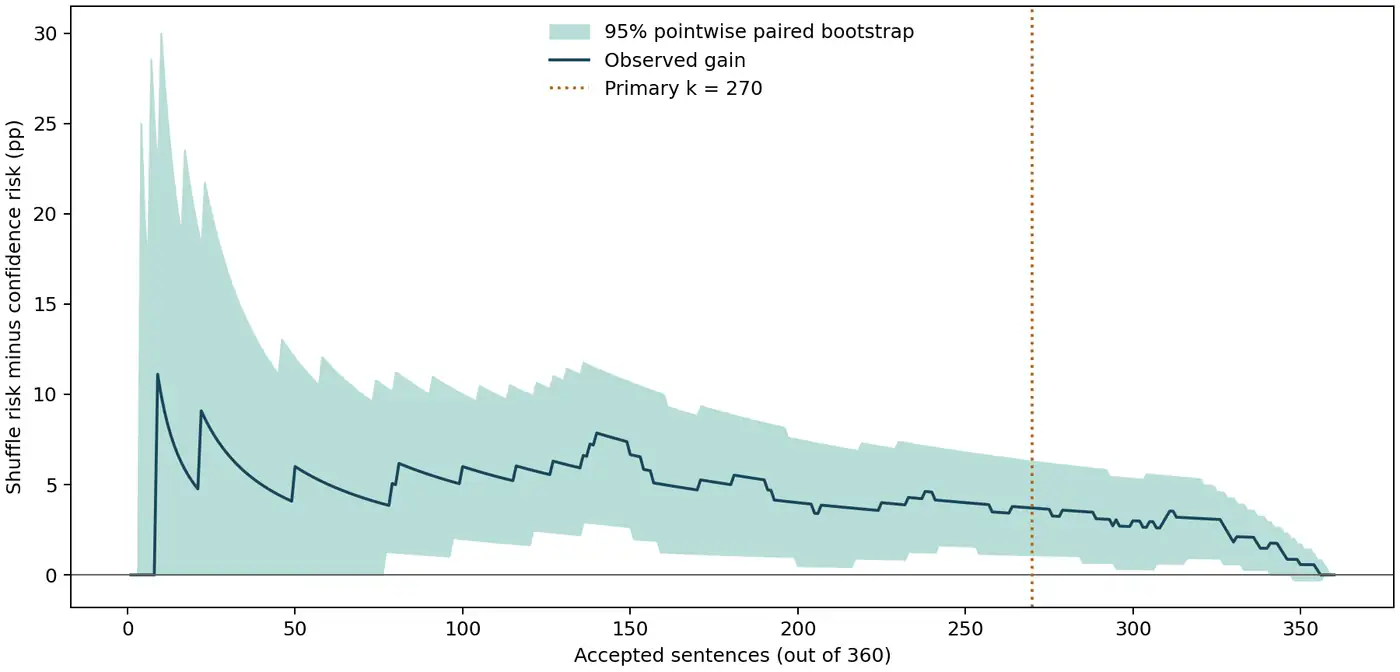
The estimation of the points in the three positions of 18, 36, and 90 gives almost the same impression, but the first comparison is only supported by a mistake in the disruption of the queue. One more mistake in the 18 positions, the risk changes by 5.5 or 6 percentage points; in the 90 positions, the same sentence only accounts for about 1.11 percentage points. The left side of the figure suddenly opens, corresponding to this integer step. The orange line in the figure is marked with the main comparison position. The light-colored area is drawn by the log, and it is calculated one by one along the horizontal axis.
The first and last two points are especially worthy of comparison. The far right end accepts all sentences, and the two queues contain the exact same multiset. The total number of errors for each sampling can be changed, but the two sides always change together, and the difference must be zero. Only one sentence on the far left end also gets a zero-width interval, but the reasons are completely different. The high-ranking sentences that the experience pool can repeatedly draw are limited, and the difference of 95% in the center is crowded at zero. A bug that has not yet been seen and highly convinced by the model may break this phenomenon. Taking this zero width as "the safest answer to a question", just misunderstood the amount of information of the small denominator.
Reading the official code and diagnosing failures
Read the forward function of the official classification header first. The input is a batch of tokenization numbers and attention masks. The encoder outputs the representation of each position, and the classification header takes the starting position of the sequence. AT Inference Time turns off the training mode, maps zero to negative and one as positive according to the model configuration. If the label number is exchanged, the sorting may still be the same, but the errors in the two queues have all changed. Therefore, the test run is not only the original score, but also the text abstract, identity, label and prediction categories.
This time, I will first test the eight sentences on the central processor, and then replay all 360 sentences according to the sixteen sentences in each batch. The formal inference cycle is about 126 seconds, and the peak process peak is about 946 megabytes. The maximum score difference between the test run and the archive is about 2.4 by 10 to the negative seventh power, and the categories are the same; all the official batches are the same item by item. The model and validation file multiplex the cache that has checked the summary. The next 4,000 repetitions only rearrange the saved rows, no longer invoke the encoder, and can be recalculated separately in an environment without model weights.
Next, read the two analysis scripts. The main program saves the error count and interval endpoints at each position. The independent audit rebuilds the confidence ordering from the absolute difference between the two raw scores and checks predictions against labels afresh. It counts how often each ID was drawn, then expands those counts in the original rank order. This uses the monotonic relationship verified earlier for binary classification. Draw by draw, the audit checks all 4,000 differences in error count at the primary position. It also reconstructs all 720 interval endpoints from integer frequency tables. Deduplicating a sample drawn with replacement changes its size and cutoff position. Shuffling the two sides independently would show up in the endpoint difference or in the recalculation at the primary position.
Code and instructions for reproducing the results
The fixed version has been made public, available from Source code directory enter, press Reproducing the results run, or control Where the equations appear in the official code Check the implementation.
Execute after installing the locked NumPy in the source directory:
python run.py && python audit.py
This minimum command takes the real freeze prediction as the input, generates the primary_counts.json of the difference between the points.json and the primary position of the main position, and prints the independent audit results. When you want to check the single-sentence prediction, follow the reproduction instructions to retrieve the pinned version of the model and data running model entry. The log retains the running command, process exit code, input identity and real batch shape. The reader can distinguish which step consumes the model's computing power and which step only consumes statistical calculations.
Research questions and summary
The conclusion applies to the audit pool observed under this protocol. At the prespecified budget of accepting three quarters of the cases, the gain over the fixed shuffled order remained positive under this paired perturbation. Hundreds of points on the plot share predictions, and each prefix contains the previous one. Pointwise intervals cannot guarantee that the entire curve lies inside the band simultaneously. Picking the coverage level with the largest observed gain and interpreting its interval as though that level had been specified in advance would introduce selection bias.
There is also an actual difference. There are a whole batch of sentences here, and then there are conditional sorting and precisely left 270 sentences. If sentences arrive one by one, researchers often have to fix a probability threshold first, and how many sentences they can accept will not know until the end of the evaluation. The next verifiable question is how many answers and how many errors can be left to the audit pool after selecting and locking the threshold on a separate calibration pool. This requires a new data isolation experiment, and today this risk difference curve is only for reference.
References
The search date is 2026-11-09.
- Geifman & El-Yaniv,Selective Classification for Deep Neural Networks,2017
- Distinbert SST-2 official model with tokenizer snapshot
- Stanford NLP, SST2 validation data version
- Hugging Face Transformers 4.49.0, Distinbert classification header source code
- SciPy official document, pair resampling and percentile interval
Apps by the author
I also build small tools for everyday life. Here are two of my apps:
- Daily Expense Journal: Track your income and spending, plan a budget and set savings goals. View on the App Store.
- One Small Action: Pick a small action that fits the time and energy you have today, then record how it felt and what you noticed. View on the App Store.
Find more articles and projects on my website: zffjzz.top. I’d love to hear how the apps work for you and what I could improve.