
There are a total of 360 short film reviews, and the model misjudged the emotions of 30 of them. If only 270 are allowed to answer, how many mistakes will the reader see? Disrupt the film review and then choose, this time left eighteen mistakes. Give the same model priority to answer the highest-score movie reviews, leaving eight mistakes. The two groups gave the same answer, and the selected film reviews were different. These ten errors, which are more indicative of the use of Confidence on this batch of data than reporting "abstention in the future" separately.
Separate the two questions first
Imagine putting a chip on the table every time you make a mistake. Now 90 are drawn from the 360 answer sheets that have been judged, and the wrong chips on the table will only reduce or maintain the original number. With the decline in the total number of mistakes alone, it is difficult to see whether the person who draws the card has the ability to choose. The more interesting question is, for every 100 cards left behind, how many wrong cards will you encounter? If all the correct answers are drawn, although the number of errors on the table has not increased, the remaining answers have become more unreliable.
In the previous experiment, whether the temperature parameters can be borrowed between the model or prompt template. This time, I return a clear two-class header, freeze the two output and predicted categories of each movie review, and only change which answers are visible. Readers can hand over the same prediction to two people, one is in the maximum probability, and the other only gets the number. When the two return the same number of answers, open the label to count. This controls both the model and the amount of answers.
From two fractions to two denominators
The model outputs two original scores, negative and positive, for each movie review, collectively referred to as logits. They can be negative, and they don't have to add up to one. After using softmax to normalize along the category dimension, take a larger probability as a sorting score. antiward sample, first The original score of the class is , the category number of this experimental is zero and one:
Indicates the degree to which the model is more biased to one of the two candidate categories. In the implementation, first subtract the maximum value in the line and then find the index, and the ratio of the two types of probability remains unchanged. The model still does a forward pass for all movie reviews, and abstension just reviews the screening of the output from the script. There is no reason for the model to generate abstent text here, and there is no reason to save the number of inferences for this batch of movie reviews.
have total A film review, the number set accepted by the rules is , the quantity is . Use Indicates the zero-one indication value of the event that is different from the official tag. Experience Coverage and empirical selective risk respectively
The coverage rate answered "how many cards were handed in", and the risk answered "how much was wrong in the returned card". The denominator in the two scales is the whole and the accept set. If no one gets an answer, the coverage rate is zero, and the risk cannot be defined. Writing the number of errors in the empty set as zero risk makes the rule that rejects everything occupy a false optimal position on the graph.
Which batch data is frozen and which two rules are compared
We used Stanford NLP’s SST-2 validation split. Before the project’s first predictions, sample IDs had been ordered by hash. The last 360 in that order formed the protocol’s audit pool. Two other pools of 256 examples each served exploration and calibration. We kept those splits and fitted no parameters on the calibration pool for this experiment. Earlier project work had already used this dataset and inspected the audit pool’s overall score and some threshold results. The equal-count comparison is new, but this rerun was no first look at a blinded pool. None of the three IMDb pools was used.
Before calculating the new curve, we write down the main readings: the two orders each take the first three-quarters, that is, 270. Next, look at the results of half, 90% and all of them, and save each integer prefix. The first order is sorted from high to low according to the maximum probability, and the same score is from small to large by number. The second item takes the fixed string and the hash number, and is arranged in a summary. It simulates a scrambling that has nothing to do with the label, and the number can be replayed as it is if it is fixed, without picking one from multiple mess results. Sorting with unrounded scores, the percentage in the text is for display only.
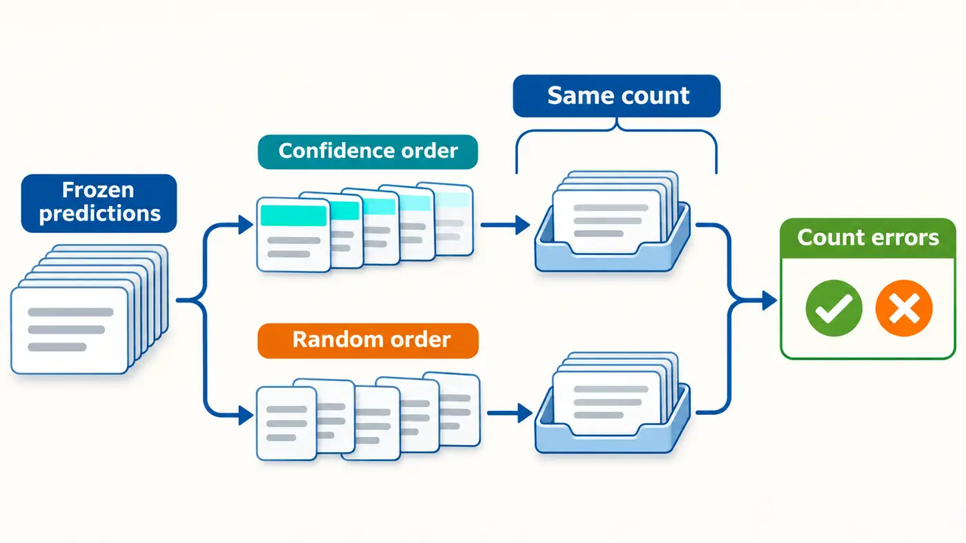
Another theoretical reference line is left. If 270 articles are drawn from 360 medium probability and non-released, each mistake has a three-quarter of the chance to be drawn. Total thirty mistakes, you will draw 22.5 on average. It is expected that decimals can be taken, and the number of errors in the actual operation must be an integer. Divide the expectations by 270 to get the full pool error rate. This reasoning is true for any positive number of acceptance, so the theoretical line is horizontal; the fixed one will move up and down. Drawing the two lines at the same time can avoid treating a precisely good disruption as a random selection of general levels.
Measured results: same answer 270 articles
| Acceptance / Total | Confidence order: number of errors / number of accepted | Scrambled Order: Errors / Accepts |
|---|---|---|
| 180 / 360 | 3 / 180(1.67%) | 12 / 180(6.67%) |
| 270 / 360 | 8 / 270(2.96%) | 18 / 270(6.67%) |
| 324 / 360 | 17 / 324(5.25%) | 27 / 324(8.33%) |
| 360 / 360 | 30 / 360(8.33%) | 30 / 360(8.33%) |
Confidence sorting is ten less than the disruption order, and the experience risk is 3.70 points lower. Calculate from the side that has not been answered again: Among the ninety articles that are suspended according to Confidence, there are twenty-two articles that would have answered incorrectly, and sixty-eight articles would have answered correctly. The disruption rules are also suspended for ninety, of which only twelve will originally have the wrong answer. If abstention is always correct, the fact that sixty-eight correct answers have been detained will be lost. If abstention is always considered a mistake, it will introduce a price that is not defined in this experiment. Readers can give the price according to their own problems, but they should keep these integers first.
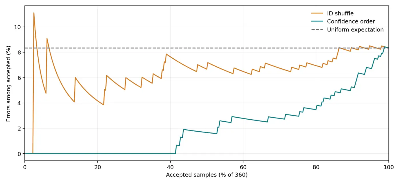
Read the picture from left to right, that is, put the answer sheet back one by one. The first 149 articles sorted by Confidence are all correct, and the first error occurs in Article 150. Its number is 544, and the probability of the model giving a larger category is about 0.99966. Seeing this, and then looking back at a zero value at the left end of the horizontal axis, you will know why you can't announce that you have found a safety threshold. That endpoint can only be positioned after reading the tag; for another criticism, the first error may appear earlier.
Each tooth in the curve has a simple explanation. Adding a correct card raises the denominator by one and leaves the numerator alone. Adding a wrong card raises both by one. As more answers are accepted, the error count can only stay level or rise, while the error rate can move either way. The selected rows in the table show the overall trend. Saving every point lets readers check the dips in between. Adjacent positions share all the earlier cards, so treating them as hundreds of independent trials would overstate the evidence. The figure has no confidence intervals, and the shuffled curve supplies neither an upper nor a lower confidence bound.
The fixed threshold is answered by another question
Another way of reading: only answer when the maximum probability reaches the pre-specified threshold. When the threshold is taken at 0.5, the probability of the second classification must reach at least half, and this time it will all be accepted. The threshold is 0.9, and 343 articles and 23 faults are accepted, the coverage rate is about 95.28, and the acceptance risk is about 6.71%. Raised to 0.99, there are still 304 crossing lines, of which 14 are wrong, and the risk is about 4.61%. The threshold is taken once, the number of acceptances is zero, and the program records the risk as a null value. All four conditions are reserved according to the original plan.
Thresholds tell us whether each film review can cross the line alone; the fixed number tells us which ranks in this review. If there is another batch of short sentences, the same threshold may accept a completely different number, but the first three-quarters will have to wait until the whole batch is sorted to be meaningful. The two rules cannot be seated directly by the same percentage. In particular, the threshold of 0.99 neither automatically reduces the error rate to one percent, nor does the coverage rate equal to 99 percent. Using this industry as a risk commitment for a new review requires additional data and agreements.
Official code reading and minimum reproduction
Look at the label mapping of the model configuration first, and then look at the DistilBertForSequenceClassification of Transformers. The encoder gives the hidden vector at each position, and the classification head takes the first position, and passes the pre-classified linear layer, activation, random inactivation layer and final classification layer. Turn off random inactivation in review mode. The batch output has two columns, and each row corresponds to one input. If the normalization axis is miswritten as a batch axis, the probability of a film review will change with other movie reviews in the same batch. In addition to the shape check, there are independent recalculation line by line, and such problems can be found directly in the fractional layer.
The model and Tokenizer use the same fixed version, the data file summary and the text abstract of each review are respectively checked. This time, I will use eight short sentences to test the CPU on the CPU, and then replay all 360 articles according to the original batch size of 16. The two original scores of the whole pool replay are the same item by item as the historical document. The forward phase uses single precision and four calculation threads, no training, no tempperature scaling . The timing includes batch tokenization, forward and extraction results, the entire pool is about 1.48 seconds. The reused resource cache is reused, and the download and installation time is not included in these two numbers.
Code and instructions for reproducing the results
The fixed version has been made public, available from Source code directory enter, press Reproducing the results run, or control Where the equations appear in the official code Check the implementation.
Execute in the source directory python run.py && python audit.py You can get two point-by-point curves, corresponding numbering sequence, fixed threshold table and independent verification results. When only these statistics are recalculated, the Python standard library is enough; if you want to replay the model from the original sentence, install fixed dependencies, obtain locking weights and verification division according to the instructions, and then perform eight trial runs and the entire pool replay. There are only derived predictions and identity abstracts in the package, and the original sentence is obtained by the data card portal. The drawing script of the drawing is read-only saved curves, so that you don't need to run the model again to change the legend or color.
Failure Troubleshooting and Research Borders
When reappearing, check the identity first, and then look at the indicators. If the number of lines is the same and the total number of errors is the same, it may still be the wrong line number for the original number as the filtered line number. The source code first compares the complete sequence of the audit list, and then checks the mapping of predictions and labels. The independent script re-estimates the probability from the difference between the two original fractions, uses the size relationship to predict, and then sums each prefix directly. It does not call the cumulative function of the main program; both paths give the same result for all seven hundred and twenty-two points and four thresholds. Readers can also check which prefix the same number is in for the first time, and locate the specific order difference.
This execution also encountered an environmental problem: the old temporary environment can find the interpreter, but the first import lacks the deep learning framework; after restoring the interpreter configuration, the tokenizer still cannot be imported. We reinstall the fixed dependencies of the records, keep the failure log, and do eight real model test runs. This sequence has practical significance: the statistical script can only show that the old score can be recalculated, and cannot prove that the current interpreter can tokenize and run the classification header. Conversely, the normal output of the model cannot prove that the accumulator handles the empty acceptance set correctly, and both checks have their own failure conditions.
In the paper, Geifman and El-Yaniv set the selection function outside the classifier, and study how to control risks under the sampling hypothesis. They examined the relevant algorithms on the visual classification data. This experiment borrows the definition of risk and coverage, and only measures the empirical curve on the fixed text pool. Based on this, the author infers that the maximum probability contains useful error sorting information in these short film reviews; the existing results are not enough to explain that these errors come from negative sentences, satire or original label differences. To explain the phenomenon of language, it is necessary to define the category, sampling method and manual judgment process first, and you cannot label the film review with just a few numbers.
Summary and testable next steps
On this audit pool, using the same classification head and accepting the same number of answers, selection by confidence made ten fewer errors than the fixed shuffled order. There was also a cost: cutting visible errors from thirty to eight meant withholding sixty-eight answers that would have been correct. A follow-up could freeze the examples, answer count, and tie-breaker, changing only the ranking score. If two scores are monotonic transformations of the same quantity, they should yield exactly the same accepted set when ranked in the appropriate direction. If they differ, check finite precision and tie handling before attributing the difference to model ability. The next experiment can test that prediction directly.
References
The following first-hand data is searched on 2026-11-07.
- Geifman, El-Yaniv, 2017, the definition of risk and coverage rate is shown in Section 2, and the risk control algorithm is shown in Section 3. Selective Classification for Deep Neural Networks
- Hugging Face, Distinbert SST-2 English Emotional Classification Checkpoint and Model Card. fixed model version
- Stanford NLP, SST-2 validate files and data cards. Fixed Data Version
- Hugging Face Transformers, Distinbert Category Header and Forward Process. The official implementation of fixed submissions
Apps by the author
In addition to writing a research blog, I also independently developed two daily tools. Daily Expense Journal Used to record income and expenditure, and arrange budget and savings goals. View on the App Store. One Small Action Let you choose a little thing according to the current time and energy, and write down your feelings when you are done. View on the App Store. If you want to continue reading technical articles, or learn about other personal works I do, welcome to visit Author personal website.